This chapter covers
- Moving, rotating, and scaling prims on the scene.
- Analyzing, creating, and manipulating meshes.
- Applying materials to prims.
- Manipulating materials for enhanced visual effects: shaders and textures.
- Exporting and importing materials between scenes: maintaining consistency and reusability.
In this chapter, let’s walk through
In the last chapter, we explored how to set up a new scene using the fundamental building blocks: Stage and Prim. We learned how to import and export scenes, providing a solid foundation for creating and manipulating 3D environments. However, merely importing assets will not make a perfect scene. In most cases you will need to move the object around, resize it, or even assign materials to improve the object’s appearance in the scene.
Therefore, manipulating the prims in an OpenUSD is essential to achieving a polished and visually appealing environment. This involves adjusting the position, rotation, and scale of objects, customizing materials and textures to enhance realism, and incorporating elements that add depth and context to the scene. Mastering these techniques will enable you to create dynamic and immersive 3D worlds that meet the specific requirements of your projects.
As an example, imagine you were building the kitchen scene we discussed in the previous chapter. You’ve already imported multiple objects such as the oven and the refrigerator and set their position and scale in the scene. However, you’ve just found a nice 3D model of a toaster that you would like to use, and when you import it, you discover a couple of problems: it is located in the middle of the kitchen floor, it is the same size as the oven, and its color doesn’t match the kitchen as well as you thought it would. Clearly, you will need to start manipulating the toaster model so that it fits correctly into the existing scene. In this example, you would alter values that determine the toaster’s scale to make it an appropriate size, adjust the values that determine its location to have it positioned on top of a work surface, and adjust values that are set by the toaster’s material properties that would vary the toasters color to match the rest of your kitchen.
We will use simple geometries and materials to provide a brief overview of the complex transformation mechanisms used in 3D programming. We will focus on understanding the basic concepts of translation, rotation, and scaling, as well as how to retrieve transformation information from 3D objects. However, a more detailed discussion of the mathematical principles behind these transformations will be reserved for a later chapter of the book. In addition, we will also examine what constitutes a material in a 3D context and how to create and apply them in OpenUSD. We will do this first by creating a simple mesh describing a flat plane, then adding to it a basic material to change its color. Later we will begin to apply more detail by adding a single texture, then by the end of the chapter, we will guide you through creating a material with multiple textures to craft a realistic looking piece of jewelry.
Let’s start with an overview of the elements that constitute a prim.
4.1 Dissecting a Prim
Let’s start with a deeper dive into the components that make up an object in a 3D scene: Xform (transform), Mesh (geometry), and Material (visual). Figure 1 provides a visual representation of these components, which we will discuss in detail.
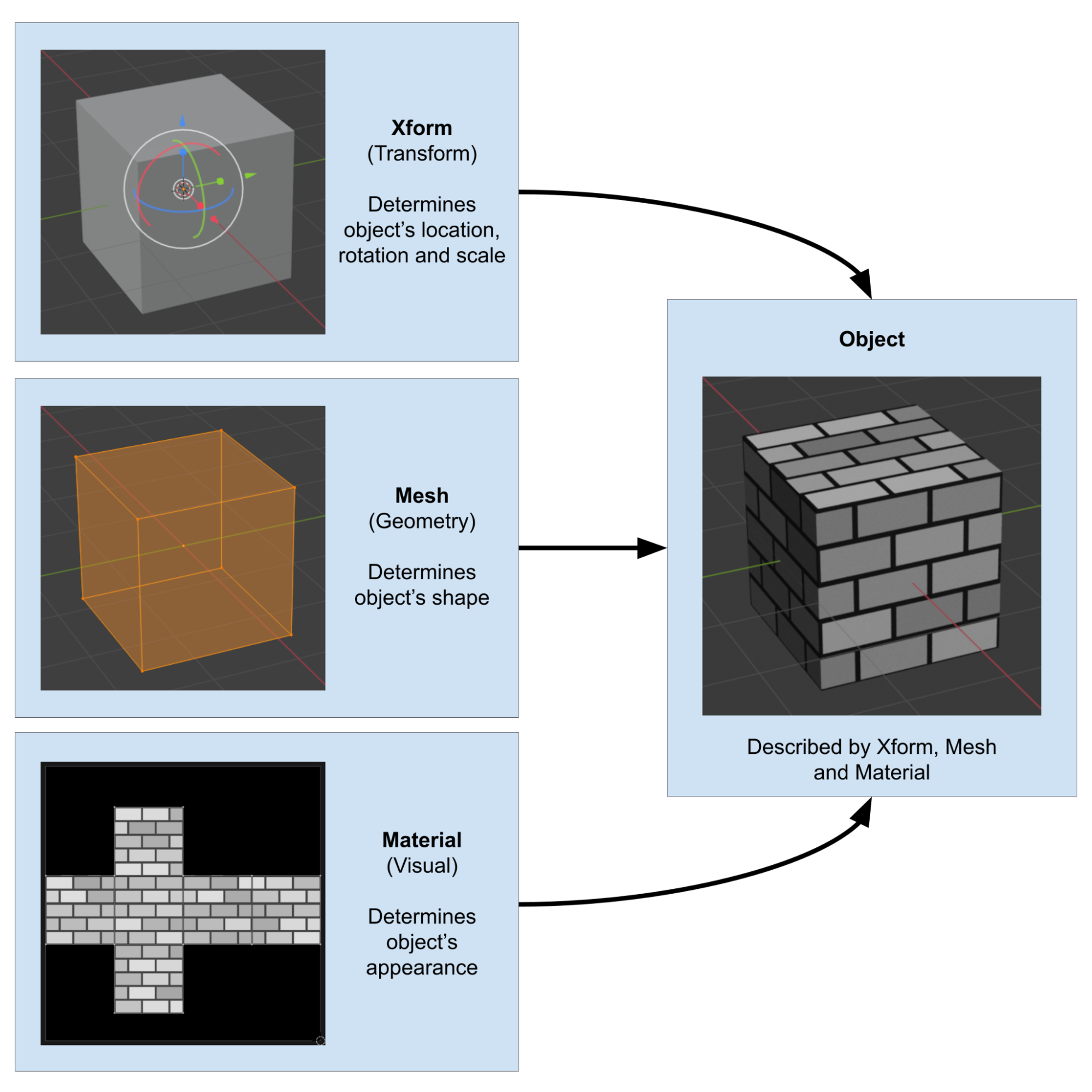
Figure 1:The three key elements that make up an object in an OpenUSD scene: Xform, Mesh and Material
These components will affect your prims in the following ways:
Xform: The transform component, described by the Xform prim, is responsible for positioning, orienting, and scaling objects in the scene. It includes properties such as translation (location), rotation, and scale. By manipulating the transform component, you can control the object’s location and relative size within the 3D environment.Mesh: The geometry component, or the Mesh prim, defines the shape and structure of the object. It consists of vertices, edges, and faces that form the object’s surface. By modifying the geometry, you can create various shapes and forms, from simple primitives to complex models. The mesh’s faces serve as a canvas for mapping materials, referred to as a UV map.Material: The visual component, or the Material prim, determines the object’s appearance by defining its surface and volumetric properties, such as color, roughness, and texture. Materials play a crucial role in creating realistic and visually appealing 3D scenes. By mastering materials, you can control the object’s visual qualities, such as reflectivity, transparency, as well as how it responds to lighting.
Imagine a scene showing a vase on a table: The Xform will determine the vase’s position on the table; the Mesh will determine its shape; and the Material will determine its color and surface texture.
Having established that a 3D object requires these three fundamental elements in order to be fully described in a scene, let’s look at each of them in more detail, starting with the Xform.
4.2 Adding a Transform
The Xformable prim, which serves as the base class for all transformable primitives, enables the encoding of arbitrary sequences of component affine transformations. These transformations can take three forms, the translation or location, the orientation or rotation, and the scale or size. Using the analogy of the vase again, its Xform will define a position on each of the three spatial axes (x, y, and z), its rotation around any of these axes, and the vase’s size using the scale parameter.
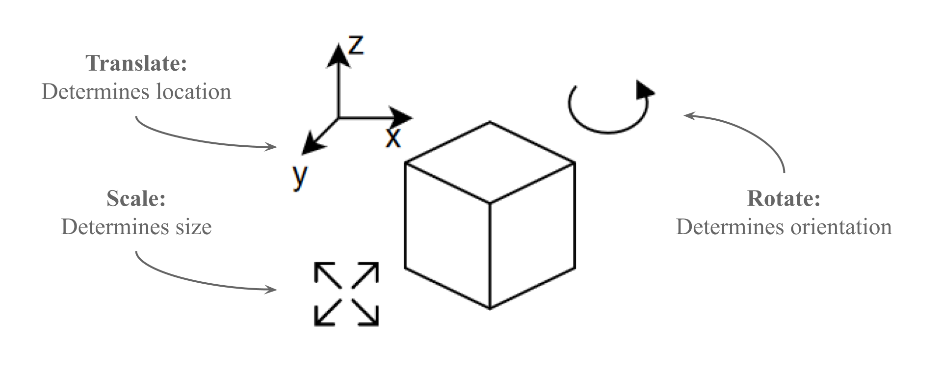
Figure 2:The three key elements that make up a transform (Xform): translate (location), rotation (orientation), and scale (size).
To position an object in a scene with a specific location, orientation, and scale, it can be placed under an Xform prim (see Figure 2). This allows you to assign transform properties, enabling precise control over its position, rotation, and size within the 3D environment.
As part of the OpenUSD framework, the Gf (Graphics Foundations) package offers a comprehensive set of geometric functions and classes that enable developers to efficiently manipulate and process 3D data, including points, vectors, and matrices.
With the following snippet we will create a new stage and reference an external prim. In this case we’ll use the cube.usda located in the ‘Assets’ folder, and then apply some transforms to it using the Gf package. We’ll use Gf.Vec3d which is a class representing a 3D vector with double precision.
After importing the modules, creating the stage and setting the defaultPrim, we’ll define an Xform type object as “object_prim”, then we’ll use the AddReference() method to assign an external reference to it. Next, we’ll create an Xform using UsdGeom.Xformable to enable transformations for the “object_prim”.
Finally, AddTranslateOp(), AddRotateXYZOp(), and AddScaleOp() are the methods we’ll use to add the transformations. The transform values are defined using Set(), and are represented as a Gf.Vec3d. In this specific example, it translates the object by units, rotates it by degrees, and scales it by a factor of along the x, y, and z axes, respectively:
from pxr import Gf, Usd, UsdGeom, Sdf
stage = Usd.Stage.CreateNew('AddReference.usda')

default_prim: Usd.Prim = UsdGeom.Xform.Define(stage, Sdf.Path("/World")).GetPrim()
stage.SetDefaultPrim(default_prim)

# Creates an Xformable object from the 'object_prim' primitive to enable transformations
object_prim = stage.DefinePrim("/World/object", "Xform")
# Add a reference to an external USD file (cube.usda) to the "object" prim using a relative path to the ‘Assets’ folder
object_prim.GetReferences().AddReference(
	"<your file path to cube.usda ex: './Assets/cube.usda'>"
	)

# Get Xformable to set translate, rotate, and scale
xform = UsdGeom.Xformable(object_prim)
xform.AddTranslateOp().Set(Gf.Vec3d(100,10,0))
xform.AddRotateXYZOp().Set(Gf.Vec3d(0,50,0))
xform.AddScaleOp().Set(Gf.Vec3d(5,5,5))

stage.Save()
Often it is useful to examine the transform data of an existing object in the scene. For example, you may want to analyse the position of an object after an action, or perhaps one object has already been rotated and now you want to precisely rotate a new object by exactly the same amount. In these cases, you would first get the transform so that you can interact with it, then extract the rotation of the original object.
Let’s use the following code to iterate through the transform operations applied to the xform prim using the GetOrderedXformOps() method (We will explore this method more fully in Chapter 6). Then we can retrieve and display each operation’s type and value. With your AddReference.usda still open in the terminal, use the following code snippet to get all three kinds of transform information from the cube:
# Iterate through transformation operations in order
for op in xform.GetOrderedXformOps():
    # Get the type of operation (e.g., translate, rotate, scale)
    op_type = op.GetOpType()
    # Get its value
    op_value = op.Get()
    print(f"Operation: {op_type}, Value: {op_value}")
This script should produce the following output:
Operation: UsdGeom.XformOp.TypeTranslate, Value: (100, 10, 0)
Operation: UsdGeom.XformOp.TypeRotateXYZ, Value: (0, 50, 0)
Operation: UsdGeom.XformOp.TypeScale, Value: (5, 5, 5)
There may be situations where we only want to retrieve one of the transforms, for example, we might just require the rotation. In this case we can directly target the specific RotateXYZOp using GetOrderedXformOps() and filtering for RotateXYZOp:
for op in xform.GetOrderedXformOps():
    # Check if the current operation is a RotateXYZ operation
    if op.GetOpType() == UsdGeom.XformOp.TypeRotateXYZ:
        rotation = op.Get()
        print("Rotation:", rotation)
        break
This script will return Rotation: (0, 50, 0), giving us only the RotationXYXOp values.
There will be occasions where you want to reset or otherwise alter the existing transform of a prim. Let’s reset the translation on the cube in our AddReference.usda stage by using the following snippet where the (Gf.Vec3d(0, 0, 0)) will define the new coordinates for the cube.
translate_op = xform.GetOrderedXformOps()[0]
if translate_op.GetOpType() == UsdGeom.XformOp.TypeTranslate:
    translate_op.Set(Gf.Vec3d(0, 0, 0))
Alternatively, the ClearXformOpOrder() method can be used to reset the transformation order on the cube, effectively removing any applied transformations without without altering the transformation data itself:
# Clears the transformation operation order, resetting any applied transformations without deleting them
xform.ClearXformOpOrder()
Transforms are invaluable for manipulating a pre-existing object within a scene. The object can be the parent of one or multiple child prims, which can enable efficient editing of objects as the transformation of a parent will percolate down to its children in the hierarchy. For example, if you have 3 cubes with a single Xform as their parent, then you are able to move, rotate or scale all three cubes at once by simply editing the data of the parent Xform instead of editing each cube in turn.
Manipulating entire objects with an Xform without altering the overall shape of the object is very common in OpenUSD, however, there will also be times when you want to work more directly with the shape of the object rather than its location, rotation or scale. In order to do this, you will need to explore its geometry.
4.3 Exploring Geometry
In OpenUSD programming, it is uncommon to directly modify mesh geometries. Usually, the mesh geometry itself is created and modified in other 3D GUIs such as Blender, Maya, or Cinema 4D. While external tools are often used for initial mesh creation, OpenUSDs framework allows for advanced geometry processing such as the creating, manipulating, and processing mesh data programmatically which helps in tasks like procedural modelling and simulations.
It is sometimes useful to be able to examine the properties of a mesh, such as its vertex points and faces, to gain insights into its structure. Understanding how to access and work with vertex and face data is essential for various tasks, such as visualization and analysis.
The three primary tasks that could be performed on a mesh are analysis, creation, and manipulation. Some examples where interaction with mesh data might be required would include:
- Analyzing a mesh: Inspecting 3D scans of manufactured parts for defects, such as in a quality control system comparing the 3D scan of a manufactured part against its CAD model to detect deviations. This would involve accessing vertex and face data to identify and highlight discrepancies.
- Creating a mesh: Visualizing anatomical structures from medical imaging data, such as in a medical application generating 3D meshes from MRI or CT scan data of organs, bones, and other anatomical structures. This would involve the creation of an accurate mesh to be used for analysis, diagnosis, and surgical planning.
- Manipulating a Mesh: Modeling natural phenomena such as fluid dynamics, weather patterns, or geological processes, such as in a simulation of riverbeds, coastlines or weather patterns. This would involve the manipulation of a mesh to reflect dynamic changes in physical models of sediment deposition, erosion, or atmospheric changes.
Let’s start exploring geometry by learning how to analyze mesh data.
4.3.1 Analyzing a Mesh
If your stage contains a mesh that you’d like to analyze, you can use the following code to retrieve its geometric information. For example, if one .usd file includes several meshes and you’re interested in knowing the number of vertices and faces for each mesh, OpenUSD provides APIs to extract this information. This can be useful for tasks such as optimizing mesh performance or ensuring that your models are consistent in terms of polygon count and vertex density.
Let’s use the cube.usda again to see the geometric components of the mesh at path /World/Cube.
In the following code snippet, we are working with the USD geometry module (UsdGeom), specifically with a mesh represented by the UsdGeom.Mesh class. First, we obtain the mesh object associated with a given prim using UsdGeom.Mesh(prim). Once we have the mesh object, we can retrieve information about the mesh’s geometry using various Get functions. The GetPointsAttr() method obtains the vertex points of the mesh, represented as a UsdAttribute. Calling Get() on this attribute retrieves the actual vertex positions. Similarly, the GetFaceVertexCountsAttr() gets the number of vertices for each face and GetFaceVertexIndicesAttr() gets the indices of the vertices that make up each face:
stage = Usd.Stage.Open("<your file path to cube.usda ex: './Assets/cube.usda'>")
prim = stage.GetPrimAtPath("/World/Cube")

# Get the mesh component from the prim
mesh = UsdGeom.Mesh(prim)
vertex_points = mesh.GetPointsAttr().Get()
vertex_counts = mesh.GetFaceVertexCountsAttr().Get()
vertex_indices = mesh.GetFaceVertexIndicesAttr().Get()

print(vertex_points, vertex_counts, vertex_indices)
The pieces of information retrieved by these methods are crucial for understanding the structure of the mesh and are often used in various mesh manipulation and analysis tasks.
4.3.2 Creating a Mesh
We’re going to create a very simple mesh representing a 2D, flat plane measuring 200 centimeters by 100 centimeters. We’ve chosen to work with a plane as it is a very simple mesh with only four vertices and one face. As you will see, each vertex has multiple variables associated with it, all of which must be set in the code. Limiting the number to four is sufficient to illustrate the mechanics of coding for meshes, without getting overwhelmed with vast numbers of variables.
In OpenUSD you define a mesh by using the UsdGeom.Mesh.Define() method and specifying its location in the scene hierarchy, for example, (stage, '/World/plane').
To give the mesh some form, we need to populate it with geometry. We do this with the CreatePointsAttr() method which defines the vertex positions. Each point, or vertex, is defined by its coordinate in 3D space (x, y, z).
The CreateFaceVertexCountsAttr() method is used to specify the number of vertices per face. In this case, the plane only has one face and there are four vertices on the face.
Next, the CreateFaceVertexIndicesAttr() method is used to define the vertex indices for each face.
Finally, the CreateExtentAttr() method sets the correct extent attribute values, defining the bounding box of the mesh. This bounding box represents the minimum and maximum corners of an axis-aligned box that fully encloses the mesh and is used to determine how the spatial dimensions of mesh will be represented in the scene, which can be useful for rendering, collision detection, and scene management calculations.
The following code snippet will create our plane as a mesh with four points and one face:
from pxr import Usd, UsdGeom, Sdf
stage = Usd.Stage.CreateNew("plane.usda")

plane = UsdGeom.Mesh.Define(stage, "/World/plane")
plane.CreatePointsAttr([(0, 0, 0), (0, 100, 0), (200, 100, 0), (200, 0, 0)])
plane.CreateFaceVertexCountsAttr([4])
plane.CreateFaceVertexIndicesAttr([0,1,2,3])
plane.CreateExtentAttr([(0, 0, 0), (200, 100, 0)])

stage.Save()
The methods above will create a mesh as shown in Figure 3.
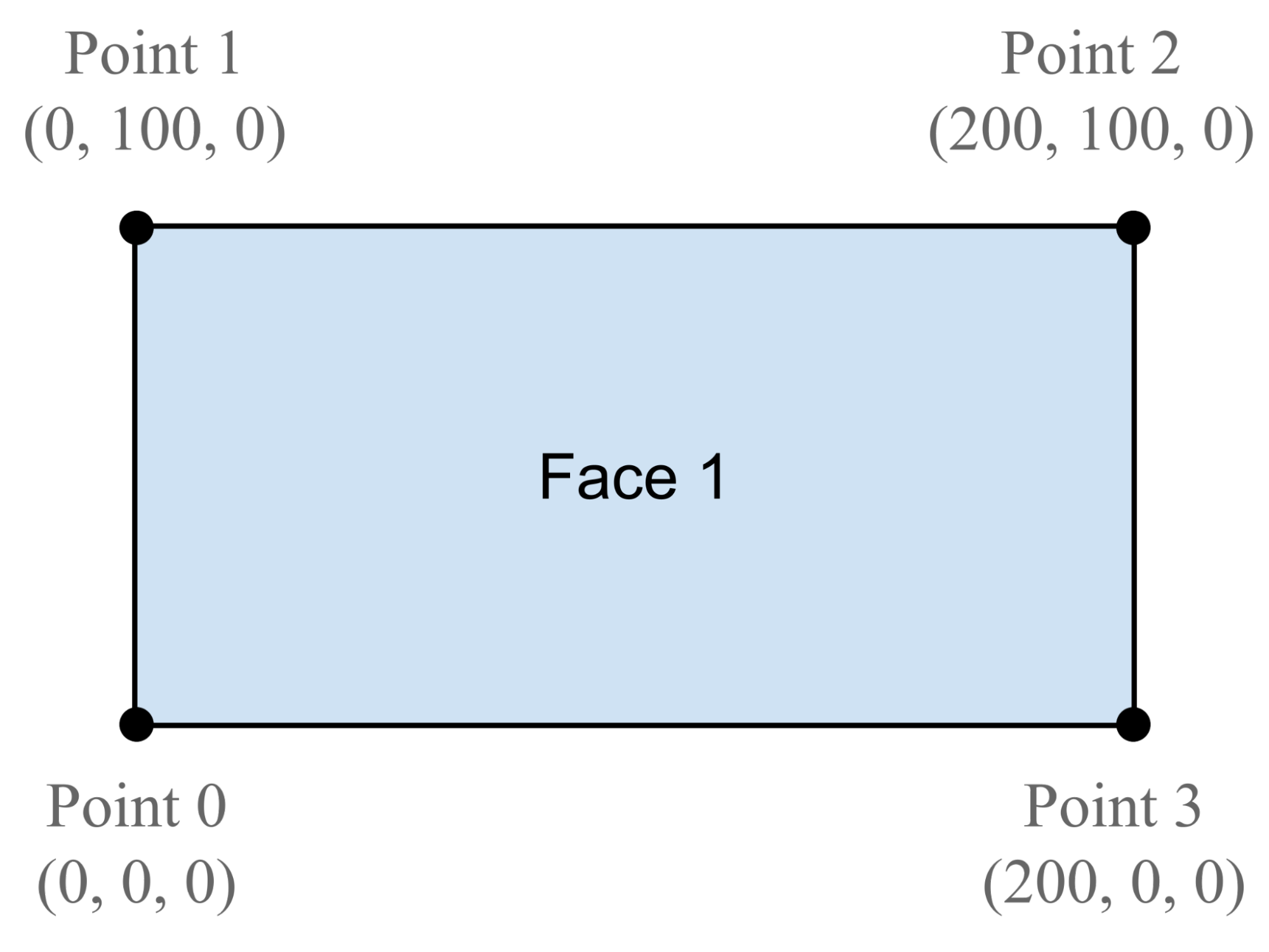
Figure 3:A simple mesh describing a two-dimensional plane. It is made up of four vertices and one face, showing the location of each vertex on the x, y and z axes. The points are numbered according to the values set by the CreateFaceVertexIndicesAttr method.
4.3.3 Manipulating a Mesh
There may be occasions where you want to manipulate a mesh. Perhaps you want to use your plane to represent the surface of a liquid or a dynamically changing landscape, or in another example, maybe you are creating a 3D bar chart whose bars will be growing or shrinking according to incoming data. In such cases, you will want to manipulate the vertices of the meshes by using the Usd.Geom module. Using the plane.usda that we’ve just created, let’s try manipulating the mesh by scaling it up by a factor of 2.
The following code will define a function ‘scale_mesh’ which takes two arguments: file_path (path to the USD file) and scale_factor. It uses UsdGeom.Mesh to retrieve the mesh from the specified path, then gets the vertex points using mesh.GetPointsAttr(). Next it scales the points by the scale factor, then alters the attributes of the existing points by setting the scaled points back on the mesh with the points_attr.Set() function.
import os
from pxr import Usd, UsdGeom

def scale_mesh(file_path, scale_factor):
    try:
        stage = Usd.Stage.Open(file_path)
        mesh_path = '/World/plane'
        mesh = UsdGeom.Mesh(stage.GetPrimAtPath(mesh_path))
        points_attr = mesh.GetPointsAttr()
        points = points_attr.Get()
        scaled_points = [(x * scale_factor, y * scale_factor, z * scale_factor) for x, y, z in points]
        points_attr.Set(scaled_points)
        stage.GetRootLayer().Save()
        print("Mesh scaled successfully.")
    except Exception as e:
        print(f"Error scaling mesh: {e}")

# Example usage
file_path = "<Path/to/plane.usda>"
scale_factor = 2
scale_mesh(file_path, scale_factor)
Program 1:Scale points on the prim
So far, we have addressed the positioning and scale of objects by using transforms, then gone on to look at the ways to work with the mesh itself. Until now, all of our objects and meshes remain an unattractive gray color, so next we will examine how to beautify them by adding materials.
4.4 Creating a Simple Material
In OpenUSD, a material is also treated as a prim. A material prim is an instance of the UsdShadeMaterial schema class, representing a reusable, abstract material definition that can be assigned to geometry. It provides a framework for organizing and binding shading properties to geometry efficiently.
Shortly, we will create a material and then go through the crucial step of binding it to the plane we just created. First, it’s worth taking some time to explore how materials work in OpenUSD.
A material prim contains a set of attributes that describe the visual properties of a surface, such as its color, texture, transparency, and reflectivity. These attributes can be seen as a collection of material properties that are applied to any object to determine its appearance. Integral to the appearance of a material, is a lower level program known as a Surface Shader, usually referred to as simply a Shader.
The difference between a material and a shader is not immediately obvious, but it can be helpful to appreciate the varied ways in which they work together to produce the final look of an object. In OpenUSD the Material Prim acts as a container for the shader and the shader calculates how the material properties will respond to the lighting in the scene. The shaders then output the computed data to be interpreted by the material prim. In short, where materials describe an object’s appearance, shaders do the computations necessary to render that appearance realistically by simulating how light interacts with the materials. For example, consider a model of a blue, glass bottle. The material and shaders will play the following roles in representing the bottle:
Material: Defines attributes such as the shade of blue, the amount of transparency and reflectivity that the glass should have, and whether the glass is worn or new looking.Shaders: Calculate how light would interact with the material’s attributes by determining how much light would pass through or reflect off the glass, given the transparency and reflectivity, and how its color would change in response to the blue color, etc.
The Material and Shader working together in this way, are referred to as the Shading Network. Table 1 describes the key differences between these two elements of the shading network.
Table 1:A Simple Comparison Between Materials and Shaders in a Shading Network.
| Materials | Shaders |
|---|---|
| A material defines the visual properties of an object’s surface (and volume if appropriate). | A shader is a program that executes on the GPU and determines how the surface (or volume) will appear when rendered. |
| It describes attributes such as color, texture, reflectivity, roughness, transparency, etc. | Shaders handle tasks such as lighting calculations, shadowing, reflections and refractions. |
| Materials provide a high-level description of how an object looks, but they don’t dictate the precise calculations involved in rendering that appearance. | Shaders operate at a lower level than materials, performing calculations to determine how light interacts with the surface (or volume) defined by the material. |
When creating a material, understanding how the various shader inputs influence the final appearance of an object is crucial for achieving a wide range of material effects and bringing realism into your scene. Therefore, before we do any scripting, let’s examine the effects that different shader properties will have on the final appearance of any object that they are bound to.
Bear in mind that the topic of material and shader properties is a huge one, which far exceeds the scope of this book. Therefore, we do encourage readers who want to get the best out of their materials to research more widely the vast amount of information that is out there. There are many established conventions in material creation and rendering that are applicable to the way OpenUSD uses materials, so any research in this area will likely improve your ability to achieve the appearance or style that you desire for your own objects and scenes. However, for the sake of readers who are not familiar with the concept of material properties, Table 2 provides a brief description of the most commonly used properties, which combined, are capable of producing very realistic looking objects.
Table 2:The Effects of Commonly Used Shader Properties
| Shader Property | Property Effect |
|---|---|
| Albedo/Diffuse | These are two interchangeable terms used for the same setting. Both are used here as they are both commonly used. It determines the base color of an object, the diffuse reflectance of the surface. The color is defined by assigning values to the red, green, and blue channels (RGB), or by adding an image which describes color variations across the surface. For example, a plain green dress could have a uniform color described by RGB values, whereas a patterned dress could have the range of colors described by an image of the pattern. |
| Roughness | This determines the minute surface irregularities of a material, influencing how light is scattered across its surface. In OpenUSD, lower roughness values indicate smoother surfaces with sharper reflections, while higher values create a more diffuse or matte appearance with softer reflections. For example, a polished metal surface would have low roughness, while a rubber tire would have high roughness. |
| Metallic | This determines whether a material behaves like a metal or a non-metal (commonly referred as dielectric in 3D shading parlance). In OpenUSD, a value of 0 indicates a dielectric material (non-metal), while a value of 1 indicates a fully metallic material. Metallic surfaces produce specular highlights and reflections, while dielectric materials do not unless they have very low roughness, such as glass. For example, a model of a coin would be fully metallic, whereas a model of a piece of jewelry might combine both metallic and nonmetallic elements. |
| Normal | Normal maps modify the surface normals of an object, simulating intricate surface details without adding additional geometry. The term 'surface normals’ refers to vectors that are by default perpendicular to the surface of an object. They influence how light interacts with the surface, and when influenced by a normal map they create the illusion of depth and detail. For example, an object representing a brick wall may be a 2D flat plane, however, by adding a normal map to the shader it can be made to appear to have individual bricks protruding from the surface that will respond accordingly to changes in lighting, giving it the appearance of being 3D. |
| Ambient Occlusion (AO) | This simulates the attenuation of ambient light based on the proximity of surfaces. It adds depth and realism to objects by darkening areas where objects intersect or are close to each other. Higher ambient occlusion values result in darker shadows, while lower values produce lighter shadows. For example, the creases on wrinkled skin would appear darker, and therefore deeper, due to ambient occlusion. |
| Emissive | This parameter is used for objects that emit light, rather than just reflecting it. It is useful for creating light sources within a scene, such as glowing signs or illuminated buttons. Emissive materials have a self-illuminated appearance and can contribute to the overall lighting of a scene. For instance, a computer monitor emitting light in a dark room would require emissive materials. |
| Opacity | As the name suggests, this determines the transparency of an object. A value of 0 indicates complete transparency, while a value of 1 indicates complete opacity. For example, a glass window would have a low opacity value, allowing light to pass through, while a solid wall would have a high opacity value, blocking light completely. |
In OpenUSD, minimum and maximum values for shader properties define the valid range of inputs that a shader can accept for a given attribute. If the attribute exceeds these values the shader typically clamps it to stay within the defined range of 0 to 1, ensuring realistic results. For example, an object with maximum opacity (1) will prevent all light from passing through it, therefore there is no reason to have values higher than 1, as no more light can be blocked. This clamping allows the rendering engine to optimize calculations, assuming values will always lie within a predictable range.
Once a material is created, it must then be assigned to the relevant mesh/s on the stage. To assign a material to a mesh, generally, you need two steps:
- Define a new Material schema class instance and set its attributes to define the desired material properties.
- Create a Binding relationship between the material prim and the mesh prim.
The Shader is the core component of the Material. The Material acts as a container for the shading network and the Shader is created as a child of the material prim. We will set the surface shader’s color, metallic and roughness properties, noting that any unset inputs will default to the values defined in the shader specification. Finally, we will connect the material’s surface output to the shader’s surface output, in this case the pbrShader, establishing the source of the Material’s surface shading.
Let’s go ahead and create a material that will turn our plane red in color. The following code will define a material and name it ‘planeMaterial’. It will also define the shader prim, and specify the properties of the shader, then create a surface output for the shader and material and connect them to each other:
from pxr import Sdf, UsdShade
# Define a material prim
material= UsdShade.Material.Define(stage, '/World/Looks/planeMaterial')
# Define a shader prim
pbrShader = UsdShade.Shader.Define(stage, '/World/Looks/planeMaterial/PBRShader')

# Define the properties of the shader
pbrShader.CreateIdAttr("UsdPreviewSurface")

# The color here is RGB color and (1, 0, 0) means total red.
pbrShader.CreateInput(
	"diffuseColor",
	Sdf.ValueTypeNames.Color3f).Set((1, 0, 0)
	)

pbrShader.CreateInput("roughness", Sdf.ValueTypeNames.Float).Set(0.4)
pbrShader.CreateInput("metallic", Sdf.ValueTypeNames.Float).Set(0.0)

# Create a surface output for the shader
pbrShaderOutput = pbrShader.CreateOutput("surface", Sdf.ValueTypeNames.Token)

# Create a material output and connect it to the shader's surface output
materialOutput = material.CreateSurfaceOutput()
materialOutput.ConnectToSource(pbrShaderOutput)

stage.Save()
The code above will create a material that is red in color. However, it has yet to be bound to any object, so let’s apply it to the plane object we created earlier.
Let’s come back to our plane (created in 4.3.2 Creating a Mesh) and apply the planeMaterial we just created to it. The following code will bind the material to the plane prim using the MaterialBindingAPI, and determine its strength relative to its descendants. The binding strength can be stronger or weaker to choose whether to cover children’s materials:
# Bind the Material to the Plane
plane.GetPrim().ApplyAPI(UsdShade.MaterialBindingAPI)
UsdShade.MaterialBindingAPI(plane).Bind(
    material,
    bindingStrength=UsdShade.Tokens.strongerThanDescendants # Set the binding strength to stronger than descendants
    )

stage.Save()
So, the code we used to create the material, then bind it to the plane will create the same material and shader relationship that is shown graphically in Figure 4. There we make a comparison between USD Composer’s Material Graph window and Blender’s Shader Editor window. You will notice that Blender uses slightly different names for some elements in the material graph, though they all perform the same function.
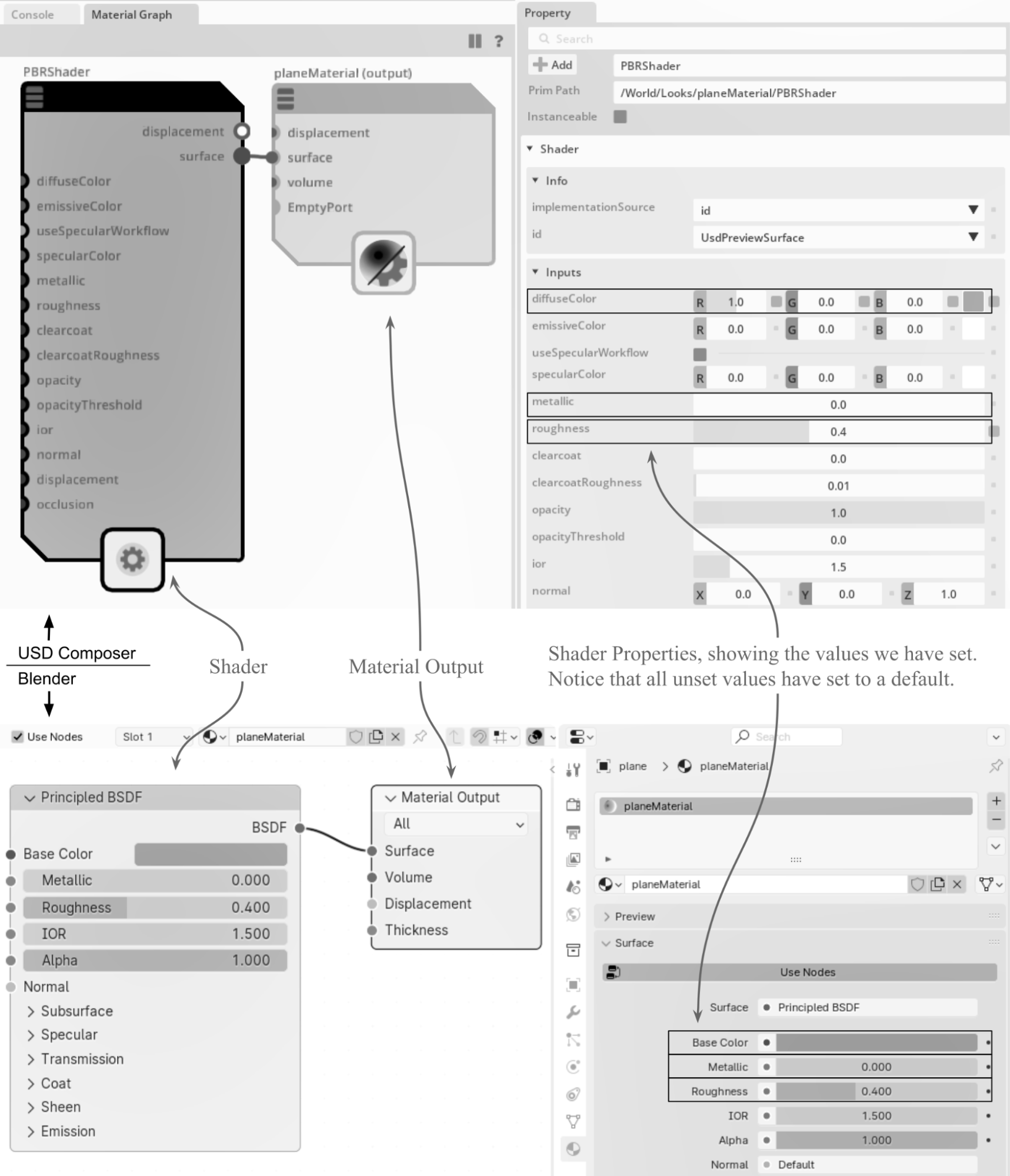
Figure 4:A graphical, node based representation of a Material and Shader pairing, as it would be viewed in USD Composer’s Material Graph window (top) and Blender’s Shader Editor window (bottom). In both cases the left panel is the Material Graph showing the shader and the material output. The right panel shows the shader properties as set by the code above. Despite the different names for some elements of the Material Graph, they all perform the same function.
Whilst creating a material with uniformly defined properties can be useful for symbolic representations of objects, such as 3D logos, cartoon characters or icons, very few objects in real life would be so uniformly colored. Therefore, if you wish to create more life-like scenes, it is likely that you will need to introduce more detail to your materials. This is commonly done by applying a well-designed image as the texture of the material.
4.5 Adding a Single Texture
Using numerical settings to adjust the color will have a unified effect over the entire surface of the object. This is fine for basic materials, such as those that would describe a brand new, single color, smooth plastic cup or a freshly polished gold ring. However, what if the cup is supposed to have a logo on it or the ring has a decorative pattern inlaid on its surface and a multi-colored, semi-precious stone? In fact, most objects we see around us have more texture, color variation, patterns and signs of wear than can be represented with basic numerical shader settings. This is when we need to ask the shader to reference an image that will provide the necessary data to give variation to the property setting and, therefore, the material’s surface. This referenced image is referred to as a texture.
Shortly, we will use code to apply a single image texture to another plane mesh like the one that we created earlier. We’ll make a new mesh, both for practice and so that you can keep the earlier one intact should you wish to review it.
4.5.1 Adding a Diffuse Color Texture
Textures can be used to influence many of the shader’s properties, replacing float values that set uniform properties across a surface with variation across a surface. In the example below, we will add an Albedo/Diffuse color as a texture. The process involves the construction of a shader network that will need to map the 2D texture images onto the mesh’s 3D surface. This requires the use of coordinates known as st coordinates, which refer to the horizontal and vertical axes in the texture space, respectively.
The st coordinates are interpreted by a UsdPrimvarReader_float2, which we will define as an stReader node. The stReader’s output is connected to a texture sampler (a UsdUVTexture sampler) that is also referencing the chosen image texture and combining these two sources of data. The UsdUVTexture sampler then outputs the combined data to the shader’s diffuse input, ensuring that the colors of the image texture override any uniform numerical values in the diffuse property. Just as before, when we created a simple material, the shader is then connected to the material output, which in turn, is bound to the desired object imbuing the object’s surface color with any variations that are present in the image texture.
To summarize, the creation of a texture shading network requires the following steps:
Create a materialOutput node: This will be the parent of each of the following shader nodes.Create a UsdPreviewSurface shader: This collates all data from other shaders in the network and is connected to the material node’s input.Create an UsdPrimvarReader_float2 shader node: This node reads the ‘st’ texture coordinates necessary for texture sampling.Set up a UsdUVTexture sampler: Connect the stReader’s output to the sampler-s ‘st’ input to map the texture coordinates.Load the image texture: Provide the texture file path to the UsdUVTexture sampler’s file input.Connect the UsdUVTexture sampler to the UsdPreviewSurface shader: Route the sampler’s RGB output to the main shader’s diffuseColor input.
Once the network is connected to the input of the materialOutput node, these steps will use the surface information to finalize the material’s visual properties, thus defining the material’s appearance on the stage.
To put this process into action, we’ll create a new plane mesh and then apply a texture to it. First, we’ll need to create the plane mesh and define the mesh’s st coordinates so that the stReader will know where to apply a texture. Next, we’ll build the shader network by introducing a UsdUVTexture sampler which we’ll name diffuseTexture, to read an image texture file. Finally, we’ll connect the diffuseTexture sampler to the surface shader’s diffuse input, which inturn, will be connected to the Material Output.
Let’s start applying a texture to a new plane mesh by importing the packages we need to assign a texture to a mesh. We will name this .usd file texture_plane.usd to differentiate it from the plane we made earlier:
from pxr import Usd, UsdGeom, UsdShade, Sdf, Gf, Vt
stage = Usd.Stage.CreateNew("texture_plane.usd")
We have already introduced most of the packages above, but you may not be familiar with the Vt library. Vt (Value Types) defines classes that provide for type abstraction and enhanced array types, which will be used later for defining texture coordinates.
Next, we can create a plane just like we did before, by defining its faces and vertices:
plane = UsdGeom.Mesh.Define(stage, "/World/plane")
faceVertexCounts = [4]
faceVertexIndices = [0, 1, 2, 3]
vertices = [
    Gf.Vec3f(0, 0, 0), Gf.Vec3f(0, 100, 0), Gf.Vec3f(200, 100, 0), Gf.Vec3f(200, 0, 0),
]

plane.CreateFaceVertexCountsAttr(faceVertexCounts)
plane.CreateFaceVertexIndicesAttr(faceVertexIndices)
plane.CreatePointsAttr(vertices)

plane.AddScaleOp().Set(Gf.Vec3f(2))  #A  make the plane twice as large for better visualization
Defining st Primvars
To apply a texture to a 3D object, we need to specify how the 2D texture st coordinates (or UV) map to the 3D object’s surface. This is done with ‘primitive variables’, or primvars.
In OpenUSD, the primvars (UsdGeom Primvars) API encodes geometric primitive variables and handles their interpolation across the topology of a primitive.
The st primvar is used to store the 2D texture coordinates for each vertex of a primitive (such as those of a cube). The st primvar is a face-varying attribute, meaning that each face of the prim can have its own set of texture coordinates.
The following code creates and sets up a primitive variable (primvar) for texture coordinates on the plane mesh:
primvar = UsdGeom.PrimvarsAPI(plane.GetPrim()).CreatePrimvar("st", Sdf.ValueTypeNames.TexCoord2fArray, UsdGeom.Tokens.faceVarying)
# Assigns st coordinates to each vertex in the order specified by faceVertexIndices
primvar.Set(Vt.Vec2fArray([(0, 0), (0, 1), (1, 1), (1, 0)]))
In the example code, the st primvar is created with a TexCoord2fArray type, which represents an array of 2D texture coordinates. The values in the array are (s, t) pairs that range from (0, 0) to (1, 1), which represent the texture coordinates.
The primvar.Set(Vt.Vec2fArray([(0, 0), (0, 1), (1, 1), (1, 0)])) assigns texture coordinates to each vertex in the order specified by faceVertexIndices that were defined when we created the plane. This is illustrated in Figure 5.
Here’s a summary of the relationship:
- Vertex 0 -> Texture coordinate (0, 0)
- Vertex 1 -> Texture coordinate (0, 1)
- Vertex 2 -> Texture coordinate (1, 1)
- Vertex 3 -> Texture coordinate (1, 0)
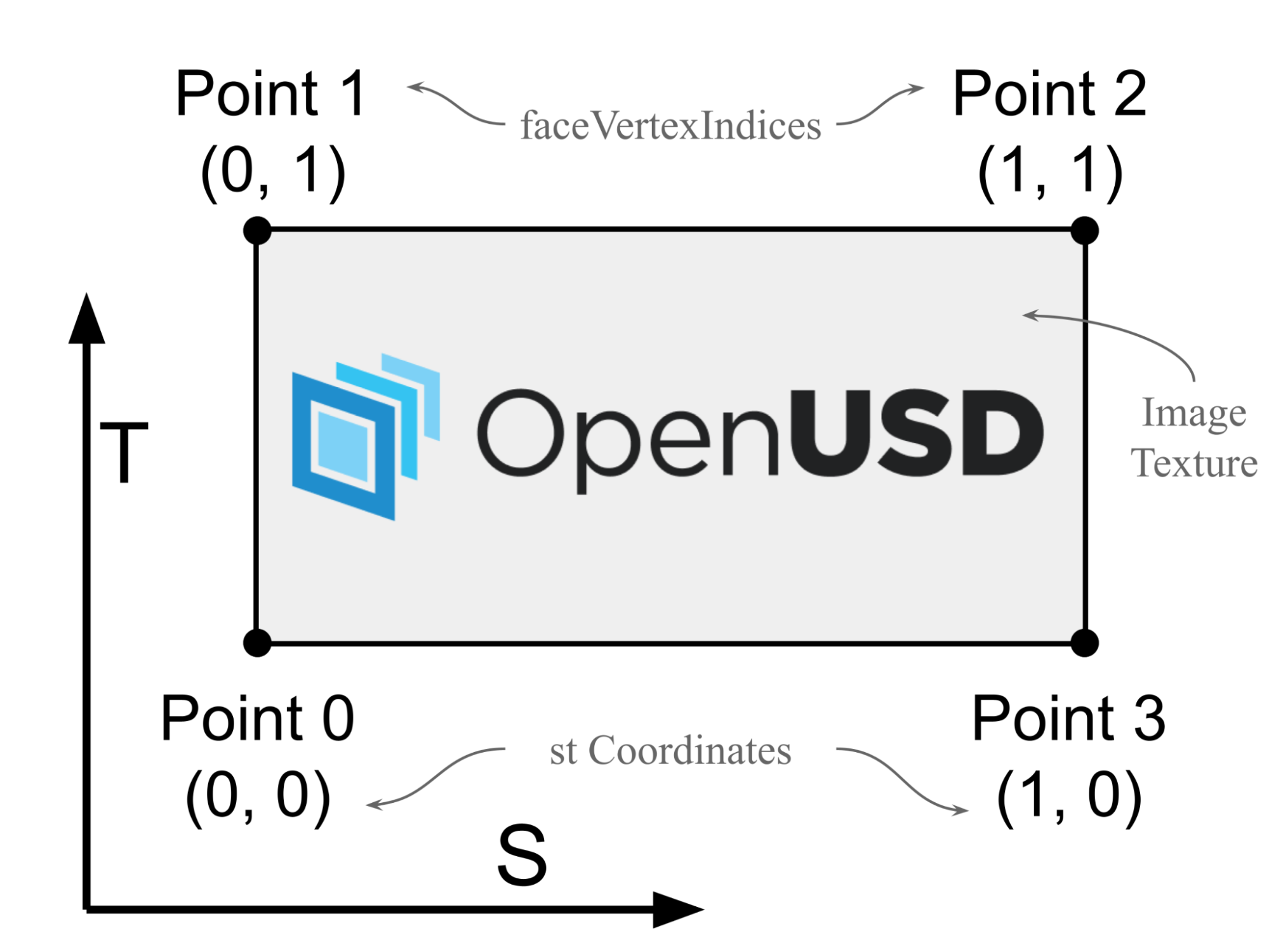
Figure 5:An illustration of texture (s, t) coordinates in texture space. The values in the primvar array are 2D vectors (u, v) that represent the texture coordinates for each vertex of the primitive. These coordinates are used to map the image texture onto the primitive’s surface, in this case, the image is the OpenUSD logo.
Having defined the st Primvars, now it is time to connect some “wires” to add a texture as the diffuse color to the plane.
Creating a Material Prim and Binding it to the Target
So far, we have created a new plane mesh and prepared it to receive an image texture at the appropriate coordinates. Now it is time to create the shader network that will display an image texture on the plane.
Let’s start by creating a material prim and binding it to the target prim:
material= UsdShade.Material.Define(stage, '/World/Looks/planeMaterial')

# Bind material to the prim
plane.GetPrim().ApplyAPI(UsdShade.MaterialBindingAPI)
UsdShade.MaterialBindingAPI(plane).Bind(material, UsdShade.Tokens.strongerThanDescendants)
Figure 6 shows the planeMaterial prim node as it would appear in USD Composer’s Material Graph window and Blender’s Shader Editor window.
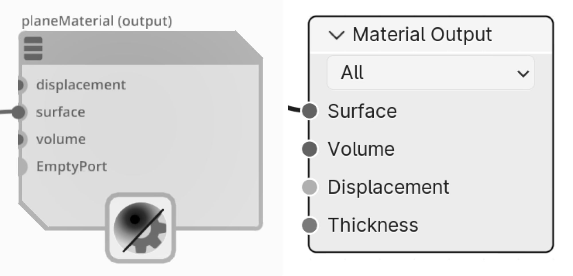
Figure 6:Material prim node created by the code above, as it would be seen in the Material Graph window of USD Composer (left) and the Shader Editor window of Blender (right).
Next we’ll create the shader that will connect to the Material Prim we’ve just made.
Creating a UsdPreviewSurface Shader
When we made the previous plane mesh and applied the material to it, we used a pbrShader. There are many different types of shader available in OpenUSD, each with different uses. The shader ID is used to identify a specific type of shader or material in a way that is consistent across different parts of a scene or different scenes. The ID helps in referencing and applying shaders correctly within the USD framework, ensuring compatibility and accurate rendering of materials in a scene. We use the CreateIdAttr() method to define the type of shader we want to use.
This time, for the sake of variation, we’ll use a UsdPreviewSurface shader. In this example project there is no specific reason to make this choice between shaders, however, we’ll use it here simply to illustrate the various options that are available.
The following code will create a UsdPreviewSurface shader named 'MainShader`, and then connect it to the planeMaterial prim.
# Create a shader as UsdPreviewSurface
mainShader = UsdShade.Shader.Define(stage, '/World/Looks/planeMaterial/MainShader')
mainShader.CreateIdAttr("UsdPreviewSurface")

# We only create a diffuse color map in this example
mainShader.CreateInput("diffuseColor", Sdf.ValueTypeNames.Color3f)
# Connect the shader to the material output node
material.CreateSurfaceOutput().ConnectToSource(mainShader.ConnectableAPI(), "surface")
Figure 7 shows the UsdPreviewSurface node, named ‘Main Shader’, as it would appear in USD Composer’s Material Graph window compared to how it would appear in Blender’s Shader Editor window (notice how Blender assigns a different name to it, though it serves the same function). The UsdPreviewSurface node acts as the central link between all other nodes in the shader network and the Material Output node. It gathers data from all connected shaders, and its ‘surface’ output connects directly to the material node’s input. This output simplifies material setup by consolidating all necessary shading information, reducing complexity, and enhancing material management within the USD framework.
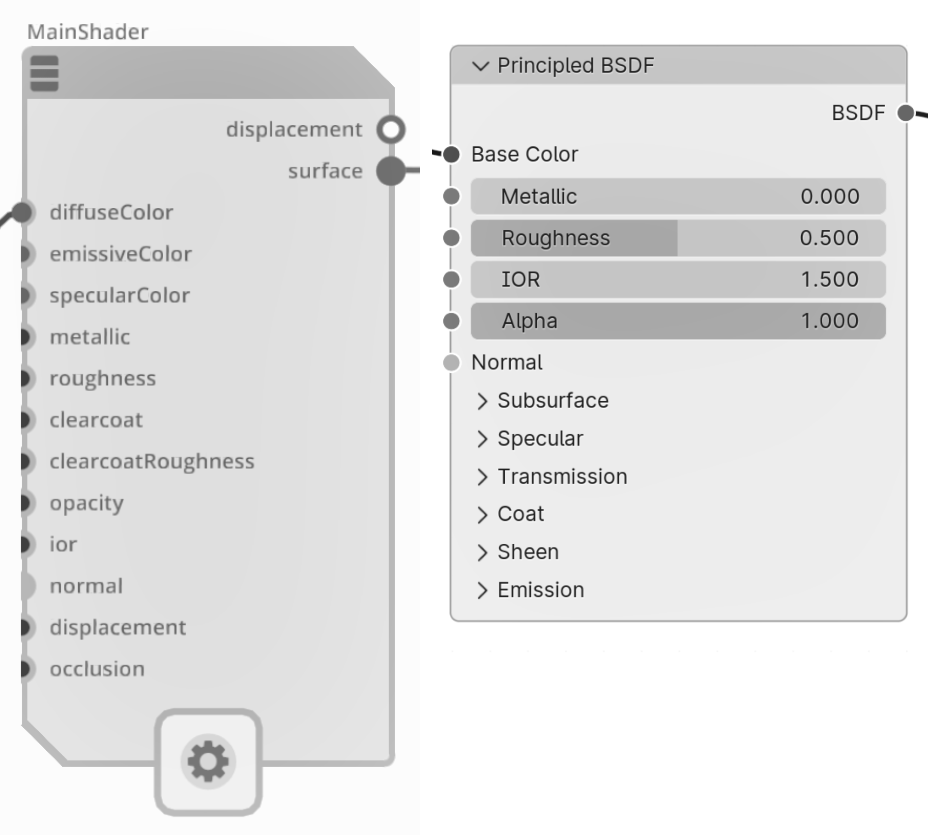
Figure 7:UsdPreviewSurface shader created by the code above, as it would appear in the Material Graph window of USD Composer (left) and the Shader Editor window of Blender (right).
Next we’ll create the node that will read the st coordinates that we set when we created the plane mesh.
Creating a Shader Node to Read the st Coordinates of a Model
The UsdPrimvarReader_float2 shader node in OpenUSD is a utility node that reads the value of a primvar from a 3D model and outputs it as a float2 value. In the context of texture mapping, this node is often used to read the st primvar, which stores the 2D texture coordinates for each point on the 3D model.
The following code will create the UsdPrimvarReader_float2 node that we will need to interpret primvars. It contains a variable called varname (variable name) which we will set to st, so that it will read the texture coordinates. We will name it stReader for clarity:
# create a shader node to read the texture
stReader = UsdShade.Shader.Define(stage, '/World/Looks/planeMaterial/stReader')
stReader.CreateIdAttr('UsdPrimvarReader_float2')
# Varname set to “st” to read the st coordinates
stReader.CreateInput("varname", Sdf.ValueTypeNames.String).Set("st")
Figure 8 shows the UsdPrimvarReader_float2 node, named ‘stReader’, as it would appear in USD Composer’s Material Graph window and Blender’s Shader Editor window.
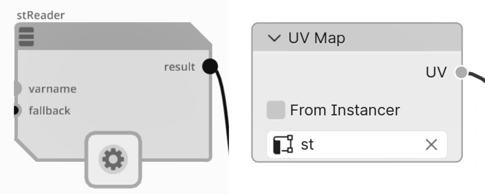
Figure 8:stReader shader node created by the code above, as it would be seen in the Material Graph window of USD Composer(left) and the Shader Editor window of Blender (right). Its varname here should be “st” to read the texture coordinates.
The stReader will need another node to connect to, which will combine the data from the texture coordinates with the data from the image texture and send it to the diffuseColor input of the UsdPreviewSurface shader. Next, we’ll create a UsdUVTexture node for this purpose.
Using UsdUVTexture Shader to Sample Texture
The UsdUVTexture shader node in OpenUSD is a texture sampling node that allows mapping 2D textures onto 3D models using st or UV coordinates. This node takes in a 2D texture image file, such as a JPEG or PNG, and samples it at specific UV coordinates to produce a color value that can be used in a shader network. The UsdUVTexture node uses the st (or uv) primvar to determine the UV coordinates for each point on the 3D model, and then uses these coordinates to look up the corresponding color value in the texture image. The resulting color value can then be used to control various aspects of the material’s appearance at different points on the model, such as its diffuse color, roughness, normal map, e.t.c.
With the following code we’re going to use UsdUVTexture shader to read an image texture that is intended to affect the diffuse color of the plane mesh. For that reason, we will name it ‘diffuseTexture’.
Let’s create the diffuseTexture shader node and name it ‘diffuseTexture’ and assign an image texture to it. We will be referencing the sample_texture.png that was contained in the Ch04/Assets/textures folder that was downloaded at the beginning of the chapter:
# Create a shader node to sample texture and name it ‘diffuseTexture’
diffuseTextureSampler = UsdShade.Shader.Define(stage,'/World/Looks/planeMaterial/diffuseTexture')
diffuseTextureSampler.CreateIdAttr('UsdUVTexture')

# Use a relative path to set the image_file_path
image_file_path = "<your file path to sample_texture.png ex: './Assets/textures/sample_texture.png'> "
diffuseTextureSampler.CreateInput('file', Sdf.ValueTypeNames.Asset).Set(image_file_path)
Figure 9 shows the UsdUVTexture node, named ‘diffuseTexture’, as it would appear in USD Composer’s Material Graph window and Blender’s Shader Editor window.
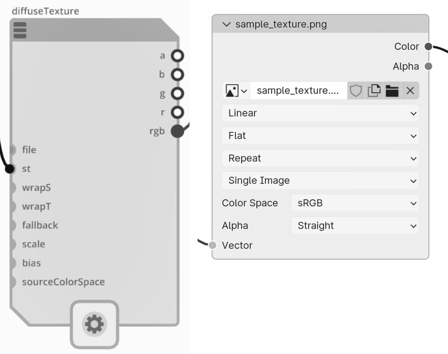
Figure 9:UsdUVTexture shader node created by the code above, as it would be seen in the Material Graph window of USD Composer(left) and the Shader Editor window of Blender (right). We should assign the “file” path to an image texture and obtain the “st” input from the stReader shader.
Next, let’s connect the stReader to the diffuseTexture shader, and the output from the diffuse texture shader to the Main Shader. To do this we first create an input and an output that we name st and rgb respectively. Then we connect the diffuseTexture output to the MainShader input:
# connect the sampler node to the reader node
diffuseTextureSampler.CreateInput("st",Sdf.ValueTypeNames.Float2).ConnectToSource(stReader.ConnectableAPI(), 'result')
# connect the diffuse texture output to the main shader
diffuseTextureSampler.CreateOutput('rgb', Sdf.ValueTypeNames.Float3)
mainShader.CreateInput("diffuseColor",Sdf.ValueTypeNames.Color3f).ConnectToSource(diffuseTextureSampler.ConnectableAPI(), 'rgb')
Finally, remember to save the stage.
stage.Save()With all the shaders connected together we should now have a functioning shader network that will be using the stReader and diffuseTexture nodes to read and combine st primvars and image textures, then passing that data through UsdPreviewSurface shader to a Material Output. When viewed in USD Composer’s Material Graph, it will look like Figure 10. As we have already bound the material output to our plane prim, the image texture will now be showing on the plane.
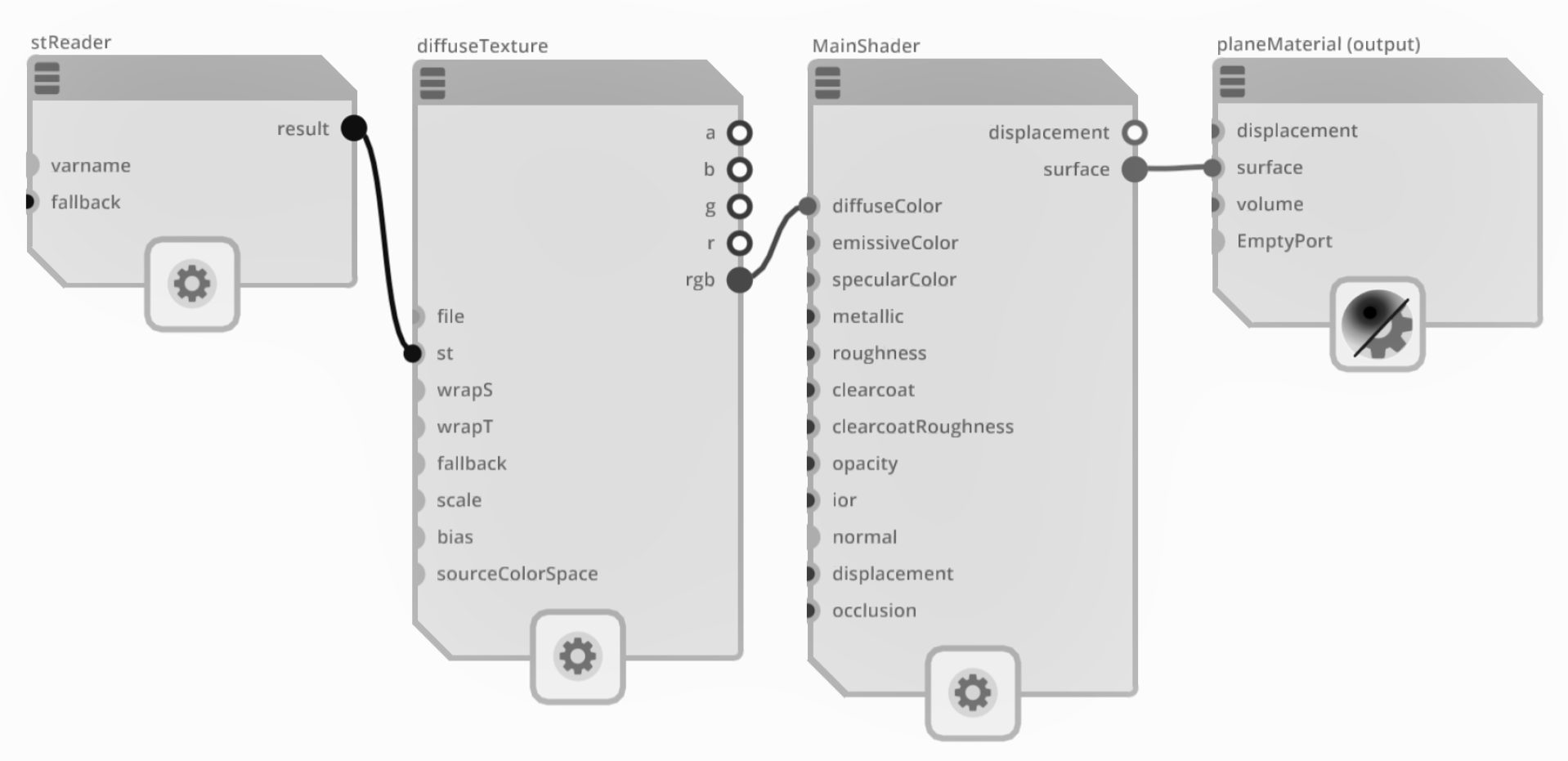
Figure 10:An overview of the shader node connections fully connected. The stReader shader node is used to read the ‘st’ texture coordinates, which are required by the diffuseTexture sampler. The image file path is then passed to the sampler’s file input. The resulting RGB values are extracted and sent to the Main Shader’s diffuse color input. Finally, the surface information is utilized to define the material’s appearance.
The resulting material is also visualized in Figure 11, which shows the texture image on the plane rendered in Blender with the Shader Editor open to view the nodes that make up the shader network. Notice that Blender transfers the OpenUSD schemas for materials and shaders into its own language, however, each node still performs the same function. A more detailed view of this will be shown towards the end of the chapter in Figure 16.
For those unfamiliar with Blender, Figure 11 also includes some instructions for navigating around the GUI and adjusting your viewpoint so that you can properly see the texture on the plane.
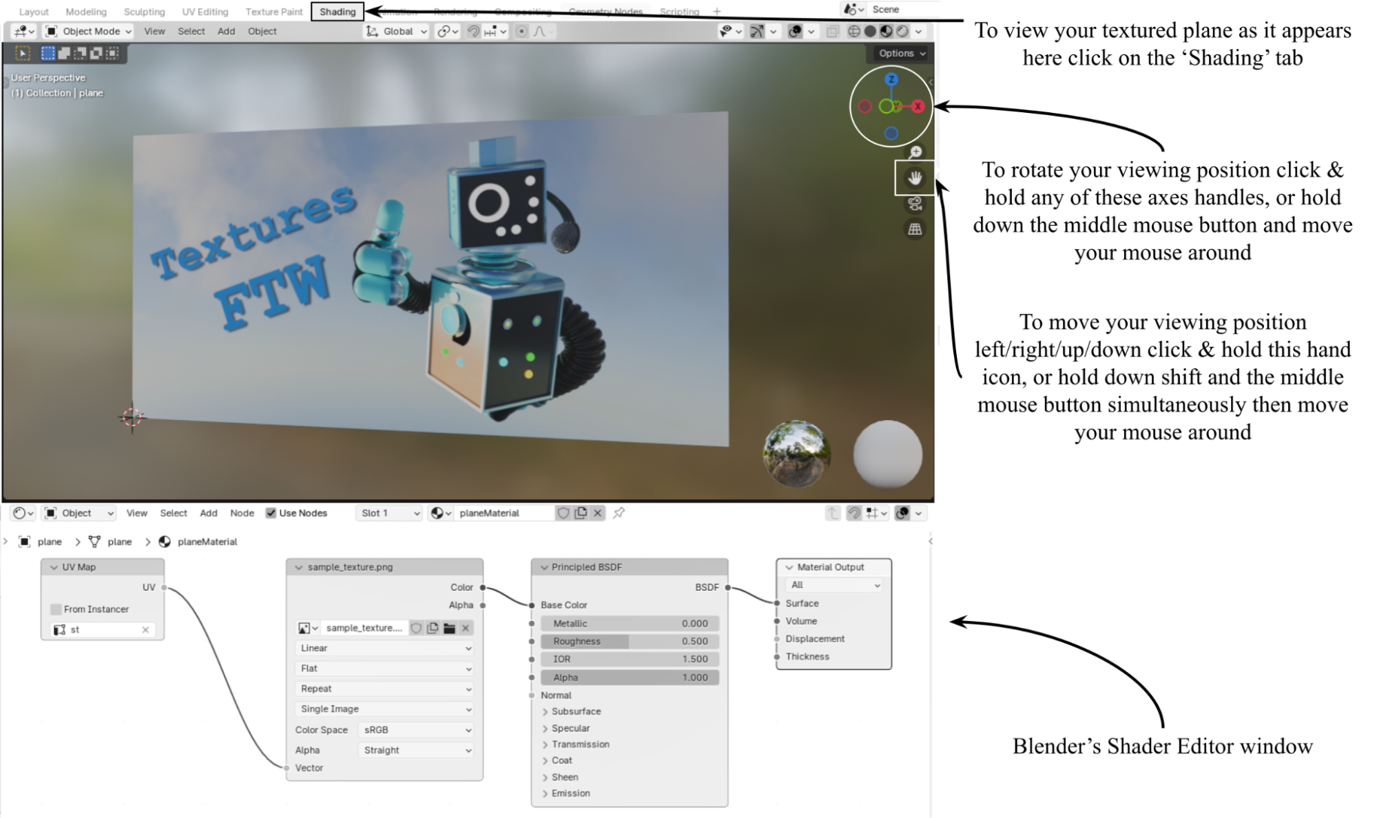
Figure 11:Visualizing texture_plane.usd in Blender using the Shading tab. The Viewport (top window) shows the image as a material on the plane, and the Shader Editor (bottom window) shows the shader network as it appears in Blender. Notice that Blender transfers the OpenUSD schemas for materials and shaders into its own language. The annotations on the right are provided for those unfamiliar with navigating around Blender.
In summary, to add a diffuse color via OpenUSD programming, we start by importing the necessary packages, including Usd, UsdGeom, UsdShade, Sdf, Gf, and Vt. We then create a new USD stage named “texture_plane.usd” and define a mesh for a plane with its faces and vertices specified. Next, we define texture coordinates using the st primvar, which stores 2D texture coordinates for each vertex. We create a material prim and bind it to the plane, and then define a UsdPreviewSurface shader to handle the diffuse color. A shader node is created to read the st primvar, and the UsdUVTexture shader node is used to sample a texture image from a specified file path. Finally, we connect the reader node to the texture sampler and the diffuse texture output to the main shader, completing the process of applying a diffuse color to the plane using OpenUSD.
However, it’s worth exploring some more complex use cases for texturing, just to illustrate the power of creating materials using this method.
4.6 Setting up A Material with Multiple Textures
In many real-world scenarios, a single texture map may not suffice to capture the full complexity and richness of an object’s appearance. To address this, we will now delve into the process of setting up a material with multiple texture maps. First, let’s explore the purpose of using multiple texture maps.
Let’s think again about that smooth, plastic cup as an example. The plastic cup with a logo printed on it would require a reference to a texture image file showing the logo and the background color of the cup. This texture image would be referenced by the Albedo/Diffuse input of the shader to represent the different colors at different points on the object’s mesh. All other input parameters, such as roughness or metallicness could remain uniform across the surface and be set as numerical inputs.
However, what if the object was a stainless-steel tankard with an embossed, polished bronze logo? It would be fine to set the Metallic input numerically to 1, fully and uniformly metallic, as all parts are metal. However, the full effect would only be obtained by adding at least three textures to other inputs. It would require an Albedo/Diffuse texture that determined the different colors of the two metals at different points on the mesh; a Roughness texture that showed the stainless steel parts of the mesh were more matt than the polished bronze; and a Normal map to adjust the normal vectors on the surface of the logo to give it apparent depth.
Multiple textures are often used to enhance realism in objects. For example, consider a well-worn toy car with scratches, dirt, and flaking paint. Some areas show the color of the paint, others reveal the underlying metal, and some parts of the paint are shiny while others are dull and scratched. By creatively applying different image textures, including diffuse, roughness, and metallic, these variations can be accurately represented, resulting in a more realistic appearance.
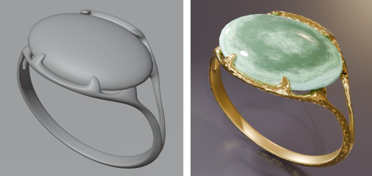
Next, we will explore how to use OpenUSD to integrate not only a diffuse color map, but also metallic, roughness, and normal maps into our material. We have created a 3D model of a gold ring with an agate stone set into it, as shown in Title Figure 12. Also, we have included four textures that, once applied, will turn it from a plain mesh into a realistic looking piece of jewelry. You will have already downloaded these assets in the Ch04 folder that we have been using throughout the chapter.
By the end of this section, you will have a good understanding of how to create a more sophisticated and realistic material with multiple texture maps using OpenUSD programming. If necessary, you may want to go back and review Table 2, to better understand the purpose of each of the textures we are about to use.
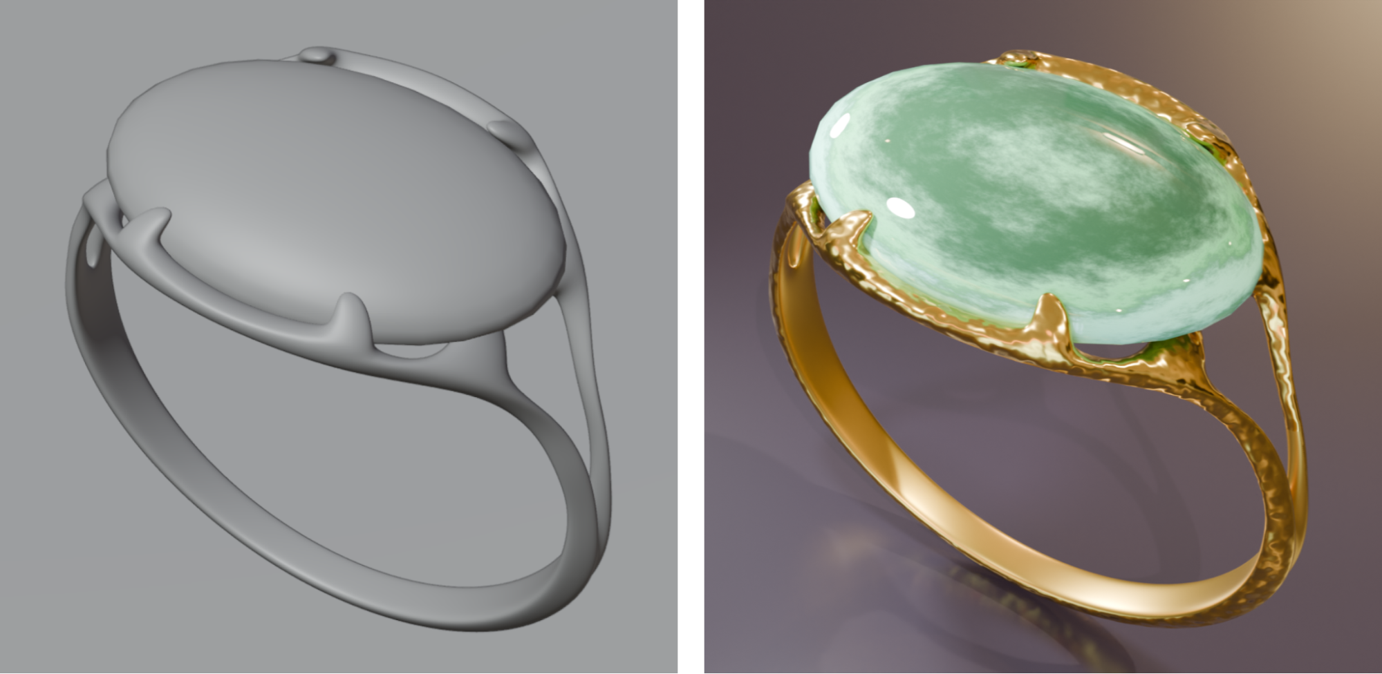
Figure 12:A model ring without any material added compared to the same model with four textures added: diffuse color; metallic; roughness; and normal.
We’re going to walk you through the process of adding textures to the unadorned mesh, until it looks much more like an actual ring made with a gold band and mounted with a polished agate stone. If you look closely at the right hand Title Figure 12, you will notice a few details, such as the smooth inside of the ring and the beaten effect on the outside (not present on the untextured model), or the more polished nature of the stone than the metal. We have chosen this model, as it has all of the elements required to show how such variation can be created by textures being interpreted by shaders.
In order to understand how the textures relate to the mesh’s coordinates, it will help to view the st (or UV) map that represents the surface of the 3D model in a 2D image. Then when you look at the various textures, you can observe where their elements map onto the mesh. Figure 13 shows the UV map that is contained in the data of the ring.usd, and which will be used by the shaders to apply the details of the textures to the 3D surface of the model. In this example we have left the UV map relatively intact, so that the shapes of the 3D model are more easily discernible. However, in most cases UV maps appear much more fragmented, as they aim to utilize the maximum amount of space available on the image, thereby achieving the best possible resolution from the 2D image.
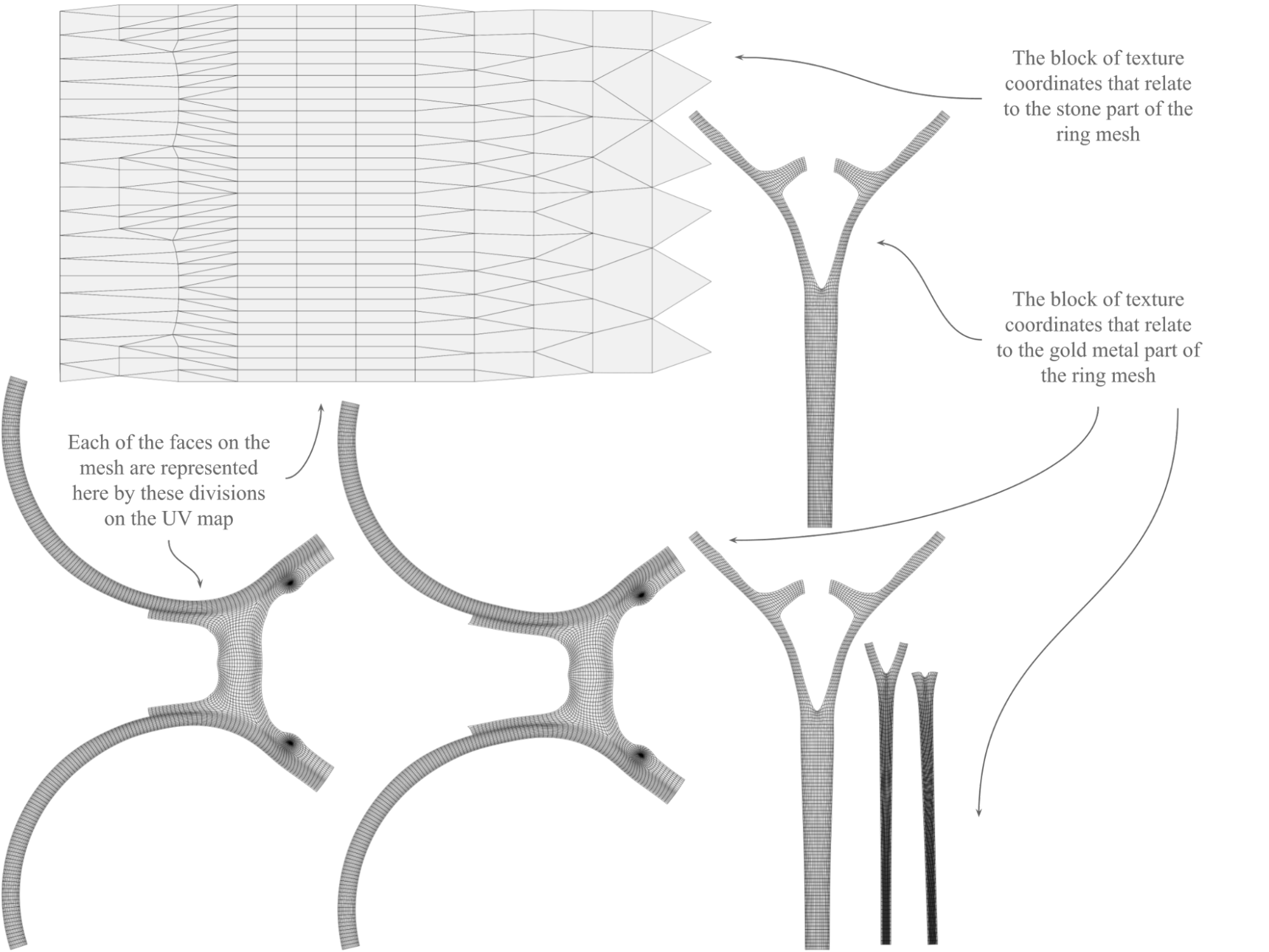
Figure 13:The map showing the 2D coordinates of each part of the 3D model, notice how the texture maps that follow add details to the same areas of the 2D image.
Each of the four textures we are going to use are shown in Figure 14 . There you can see the diffuse, metallic, roughness and normal maps and how they relate to the UV map shown above.
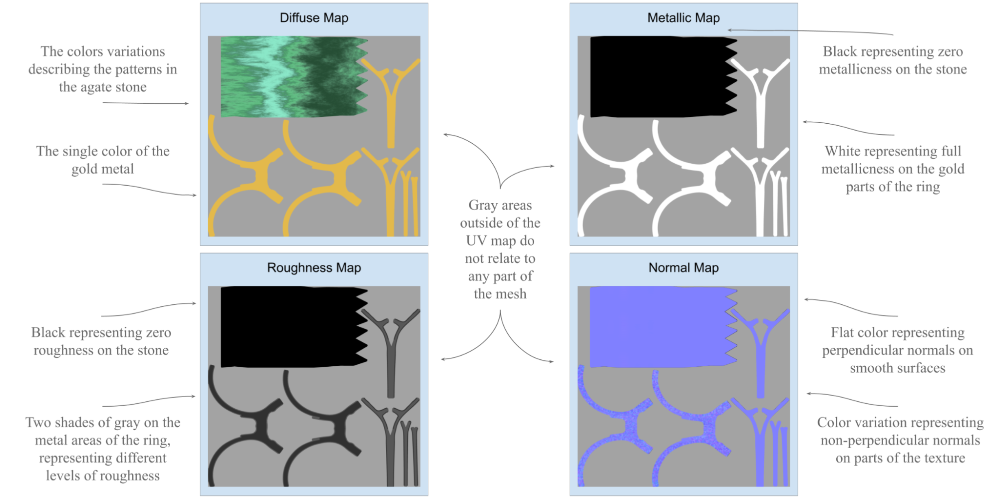
Figure 14:The four texture maps that will be applied to the ring mesh. Top left is the Diffuse map, top right is the Metallic map, bottom left is the Roughness map and bottom right is the Normal map.
Each map serves a specific purpose, let’s examine them each in turn.
Diffuse Notice how the diffuse texture is purely one color on the areas where it represents the gold band of the ring. This is because polished gold is generally uniform in color. In contrast, the area that maps to the agate stone contains all the variation you might expect to find in a decorative stone.
Metallic The metallic texture does not require color as it is only describing the degree to which the material is metallic, hence, the non-color values. Similar to how we applied a numeric value in the first plane model we made earlier, the black and white represent a float value between 0 and 1, black is non metallic, and white is fully metallic. Notice in the ring’s metallic texture, how the areas that relate to the gold band of the ring are completely white, meaning that they are fully metallic, and the stone area is fully black as it has no metallic properties.
Roughness Similar to Metallic maps, Roughness maps only require a gray scale. They represent a float of 0 to1, just as the metallic map does. Black means zero roughness, or in other words, highly reflective, whereas white means fully rough and non-reflective. Notice how the area relating to the agate is completely black, meaning that the stone has no roughness, so will appear highly polished, whereas the ring’s metal band has two shades of gray, representing slightly different levels of reflectivity on different parts of the metal band. If you look again at the ring in Figure 12, you will see that the inner surface of the band is less polished than the outer surface.
Normal You will recall from Table 2, that the normal map tells the shaders which direction light will bounce off the surface of a mesh. The normal map for our ring shows that most of the texture depicts a flat surface, meaning light will be calculated to bounce perpendicularly off the mesh. However, notice how there are some areas of the ring’s band that have a dimpled effect. If you look again at the untextured model in Figure 3.6, you will see that the untextured model has no such dimpling, whereas the textured model does. The effect serves to give the outside of the ring the appearance of beaten metal. This apparent deflection of the model’s surface is created entirely by the normal map, which is altering how the shaders calculate the angles that light will bounce off the mesh.
Let’s get started by creating a new stage, and the material and shader network that will transform the plain model into a realistic looking ring.
Creating a Material Output Node
First, let’s create a stage and call it texture_ring , create an Xform that will be the parent of the imported ring mesh, then reference the USD file containing the ring mesh:
from pxr import Usd, UsdGeom, UsdShade, Sdf
stage = Usd.Stage.CreateNew("texture_ring.usd")
# Create an Xform
ring = UsdGeom.Xform.Define(stage, "/World/Ring")
ref_asset_path = "<your file path to Ring.usd ex: './Assets/Ring.usd'>"
references: Usd.References = ring.GetPrim().GetReferences()
# Load external reference
references.AddReference(
    assetPath=ref_asset_path
)
Now, let’s create a material and bind the material to the ring mesh prim. The material will be named ‘ringMaterial’:
material= UsdShade.Material.Define(stage, '/World/Looks/ringMaterial')
ring.GetPrim().ApplyAPI(UsdShade.MaterialBindingAPI)
UsdShade.MaterialBindingAPI(ring).Bind(material, UsdShade.Tokens.strongerThanDescendants)
Utilizing a UsdPreviewSurface Shader
OpenUSD’s UsdPreviewSurface shader is a standard surface material shader used for preview rendering, and to provide a consistent look across different rendering engines. It is designed to facilitate easy material definition and interoperability within the OpenUSD framework. We will use it here as the main shader in the network.
The following code will create a UsdPreviewSurface shader as a child of the ringMaterial, and name it ‘MainShader’. Then it will create a SurfaceOutput on the shader and connect it to the surface input of the ringMaterial. This is the main shader that we will connect each of the textures to:
mainShader = UsdShade.Shader.Define(stage, '/World/Looks/ringMaterial/MainShader')
# Create a UsdPreviewSurface shader
mainShader.CreateIdAttr("UsdPreviewSurface")
# Connect the shader to the material
material.CreateSurfaceOutput().ConnectToSource(mainShader.ConnectableAPI(), "surface")
Creating a UsdPrimvarReader_float2 Shader
Next, to interpret the texture coordinates, which are Primvars, we need to create a UsdPrimvarReader_float2 node. This will load the st coordinates from the ring mesh and output them as a float2 value. We will define this node as stReader. We will only need one primvar reader node in this shader network as it will be able to load all the different texture maps:
stReader = UsdShade.Shader.Define(stage, '/World/Looks/ringMaterial/stReader')
stReader.CreateIdAttr('UsdPrimvarReader_float2')
stReader.CreateInput("varname", Sdf.ValueTypeNames.String).Set("st")
Setting Up a UsdUVTexture Sampler
Next you will need something to read the texture map. You can create a UsdUVTexture sampler node and name it diffuseTexture to differentiate it from the other textures we will be adding. Now, connect it to the mainShader diffuseColor input like this:
diffuseTextureSampler = UsdShade.Shader.Define(stage,'/World/Looks/ringMaterial/diffuseTexture')
diffuseTextureSampler.CreateIdAttr('UsdUVTexture')

diffuse_file_path = "<your file path to Ring_DIFFUSE.png ex: './Assets/textures/Ring_DIFFUSE.png'>"
diffuseTextureSampler.CreateInput('file', Sdf.ValueTypeNames.Asset).Set(diffuse_file_path)

# Connect to the st reader node
diffuseTextureSampler.CreateInput("st",Sdf.ValueTypeNames.Float2).ConnectToSource(stReader.ConnectableAPI(), 'result')

# Connect to the main shader
diffuseTextureSampler.CreateOutput('rgb', Sdf.ValueTypeNames.Float3)
mainShader.CreateInput("diffuseColor",Sdf.ValueTypeNames.Color3f).ConnectToSource(diffuseTextureSampler.ConnectableAPI(), 'rgb')
You can use exactly the same method to load the normal map. Remember, each texture will need its own sampler, so for clarity, this one will be named ‘ormalMap’:
normalMapSampler = UsdShade.Shader.Define(stage,'/World/Looks/ringMaterial/normalMap')
normalMapSampler.CreateIdAttr('UsdUVTexture')

normal_file_path = "<your file path to Ring_NORMAL.png ex: './Assets/textures/Ring_NORMAL.png'>"
normalMapSampler.CreateInput('file', Sdf.ValueTypeNames.Asset).Set(normal_file_path)

# Connect to reader node
normalMapSampler.CreateInput("st",Sdf.ValueTypeNames.Float2).ConnectToSource(stReader.ConnectableAPI(), 'result')    #B

# Connect to the main shader
normalMapSampler.CreateOutput('rgb', Sdf.ValueTypeNames.Float3)
mainShader.CreateInput("normal",Sdf.ValueTypeNames.Color3f).ConnectToSource(normalMapSampler.ConnectableAPI(), 'rgb') The following code shows how to connect a roughness map:
roughnessMapSampler = UsdShade.Shader.Define(stage,'/World/Looks/ringMaterial/roughnessMap')
roughnessMapSampler.CreateIdAttr('UsdUVTexture')

roughness_file_path = "<your file path to Ring_ROUGHNESS.png ex: './Assets/textures/Ring_ROUGHNESS.png'>"
roughnessMapSampler.CreateInput('file', Sdf.ValueTypeNames.Asset).Set(roughness_file_path)
roughnessMapSampler.CreateInput("st",Sdf.ValueTypeNames.Float2).ConnectToSource(stReader.ConnectableAPI(), 'result')

# Pick the only one (red color) channel as the output
roughnessMapSampler.CreateOutput('r', Sdf.ValueTypeNames.Float)
# Connect to the main shader via one color channel
mainShader.CreateInput("roughness",Sdf.ValueTypeNames.Float).ConnectToSource(roughnessMapSampler.ConnectableAPI(), 'r')
Finally, let’s connect the metallic map:
metallicMapSampler = UsdShade.Shader.Define(stage,'/World/Looks/ringMaterial/metallicMap')
metallicMapSampler.CreateIdAttr('UsdUVTexture')

metallic_file_path = "<your file path to Ring_METALLIC.png ex: './Assets/textures/Ring_METALLIC.png'>"
metallicMapSampler.CreateInput('file', Sdf.ValueTypeNames.Asset).Set(metallic_file_path)
metallicMapSampler.CreateInput("st",Sdf.ValueTypeNames.Float2).ConnectToSource(stReader.ConnectableAPI(), 'result')

# Pick the red color channel as the output
metallicMapSampler.CreateOutput('r', Sdf.ValueTypeNames.Float)
# Connect to the main shader via one color channel
mainShader.CreateInput("metallic",Sdf.ValueTypeNames.Float).ConnectToSource(metallicMapSampler.ConnectableAPI(), 'r')
Save the stage and you can now visualize the texture_ring.usd in your chosen viewer.
stage.Save()For a graphical representation of the shader network you have just created, see Figure 15, which shows how it would look in the Material Graph window in USD Composer.
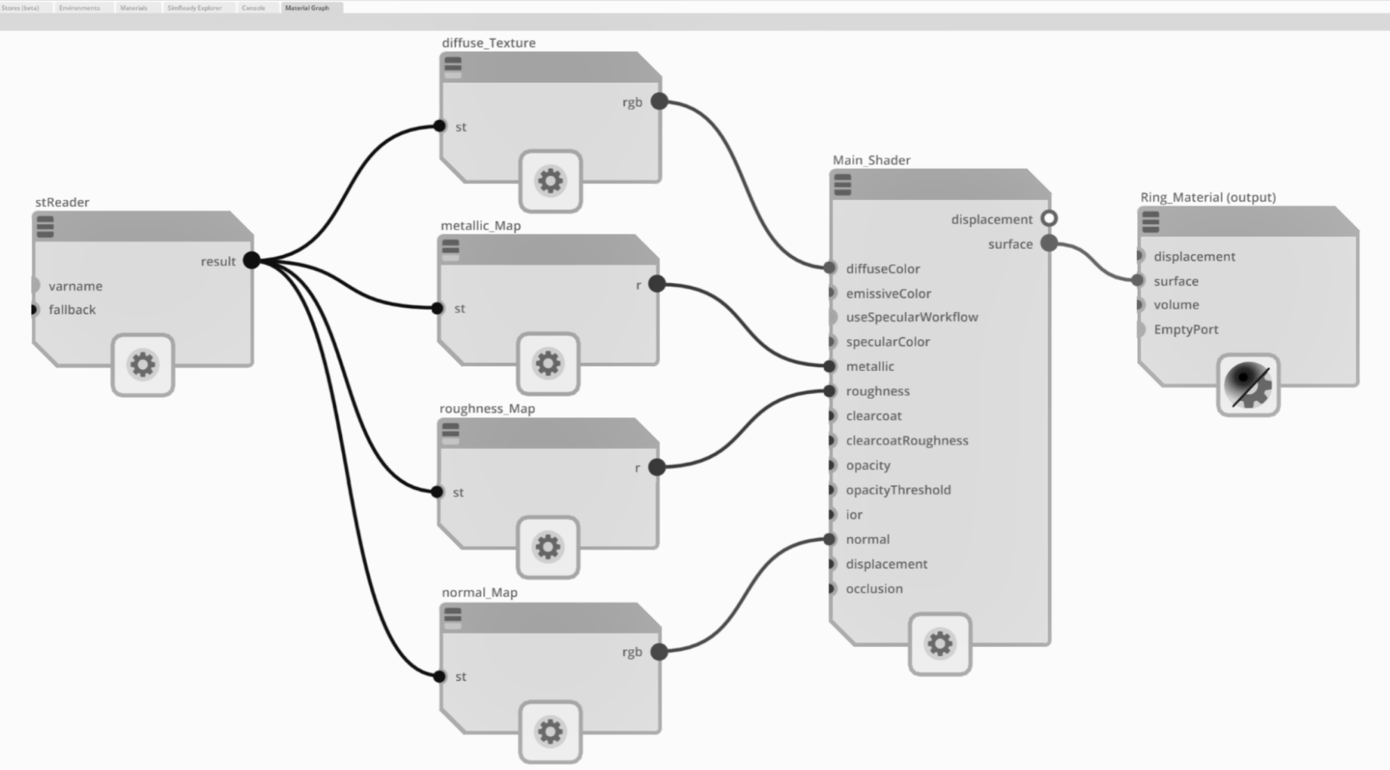
Figure 15:The completed shader node as it would appear in USD Composer, showing connections from the stReader, through the texture samplers and into the UsdPreviewSurface node. From there, the data flows to the input of the ringMaterial output node. Notice that the grayscale textures output from a single channel float ‘r’, whereas the colored textures use the float3 ‘rgb’ output.
If you are using Blender, you can view the ring with its materials added by opening the ‘Shading’ tab as we did previously to view the sample texture on the plane (review Figure 11). This will show you the materials on the ring and the Shader Editor window. However, whichever tab you are viewing in, there are other ways to view materials on objects by selecting from the four Viewport Shading modes at the top right edge of the viewport.
The default shading mode is Solid mode which shows the model as a gray object. Figure 1 shows that to the right of the Solid mode button is Material Preview mode which will show the materials on the object and provide a temporary light source which is useful when you don’t have any light present on the stage. On the far right is the Rendered mode which approximates how the scene will look when rendered. If there are no lights on the stage the viewport will remain dark. However, it is possible to use the same temporary lighting used by the Material Preview mode in the Rendered mode by clicking on the down arrow to the right of the mode buttons and unchecking the ‘Scene World’ box (remember to check this box again if you later wish to view accurately view any new lighting you add).
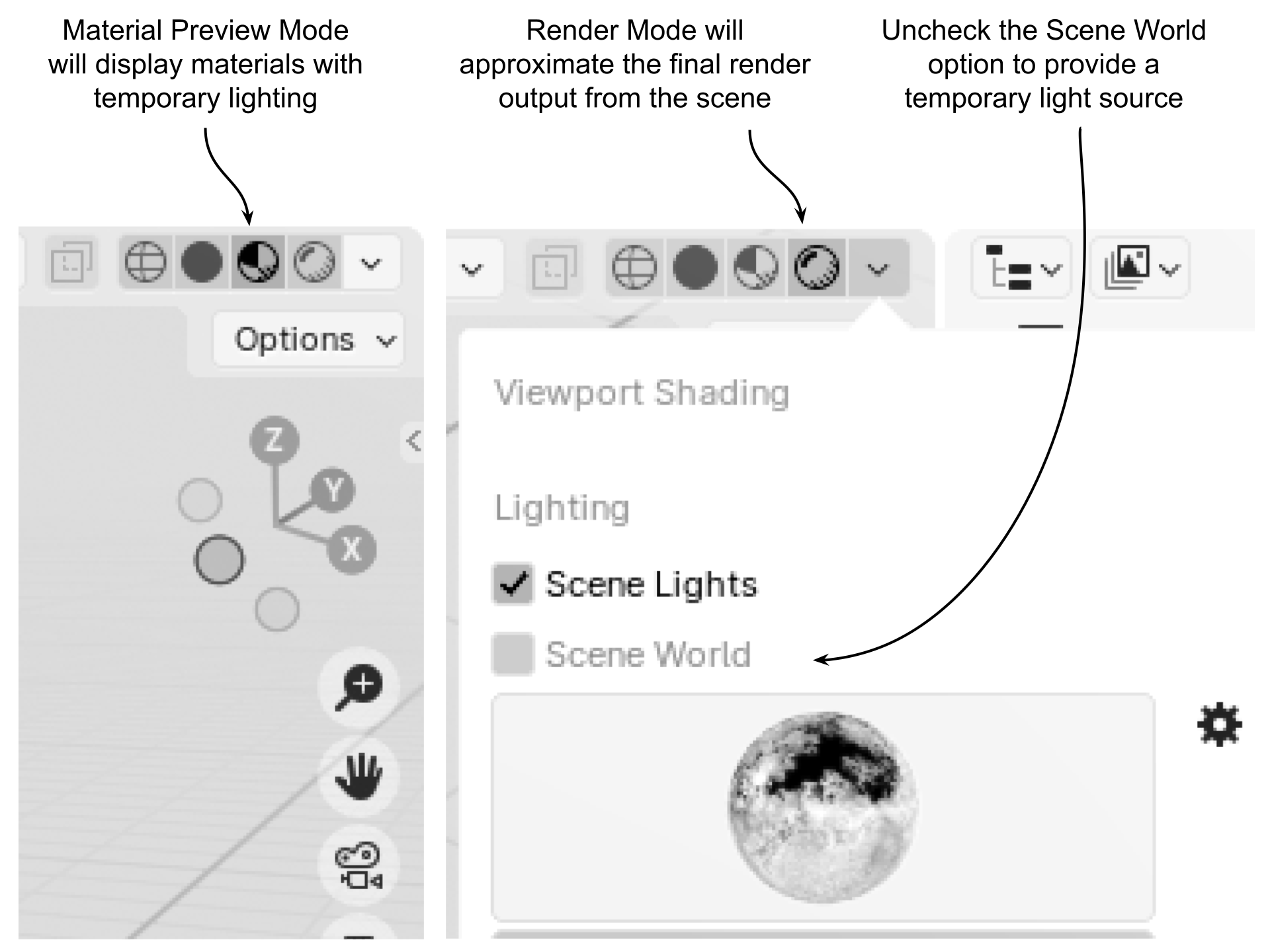
Figure 16:How to change the Viewport Shading Mode in Blender. The buttons found at the top right of the Viewport allow you to choose from various displays of materials and lighting in the viewport. The Material Preview will show materials with a temporary light source and the Render view will approximate the final render output. Render view can also be assigned a temporary light source by unchecking the Scene World option.
Figure 17 shows the shader network and the ring model as it would appear in Blender. As we saw with the plane material earlier, the network appears slightly different again because Blender transfers the schemas for materials into its own language. However, just as before, these differently named nodes all perform the same functions as those in USD Composer.
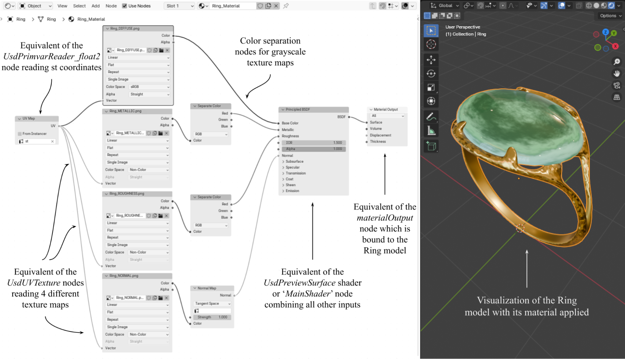
Figure 17:Visualizing texture_ring.usd in Blender. Notice that Blender transfers the OpenUSD schemas for materials and shaders into its own language. The figure shows the equivalent role that each of Blender’s nodes play.
Now that you have learned how to work with meshes, textures, materials, and shaders, and are able to manipulate your 3D objects in order to make them look exactly how you need them to, it’s time to start thinking about the next step towards getting a finished product. In many real world scenarios, it is not enough to create the 3D object and polish its appearance with materials, you also need to produce a 2D image or a video of your creation. This is where the art of setting up lighting, cameras and rendering comes in, and we will explore that in the next chapter.
Summary
- The transform component (Xform) is responsible for positioning, orienting, and scaling objects in the scene. It includes properties such as translation, rotation, and scale.
- The geometry component (Mesh) defines the shape and structure of the object, consisting of vertices, edges, and faces that form the object’s surface.
- The visual component (Material) determines the object’s appearance by defining its surface and volumetric properties, such as color, roughness, and texture via a shader network.
- Shaders calculate how the material properties will respond to the lighting in the scene, while materials define the visual properties of an object.
- Combining multiple textures into a shader network is necessary to produce realistic looking objects and helps to maintain consistency in how your materials will display across different render engines and software platforms.