This chapter covers
- Simulating physics with OpenUSD
- Understanding basic physics in OpenUSD
- Applying Rigid Bodies to objects
- Creating collisions between objects
- Using Physics Materials
- Playing with joints and articulations
One of the most exciting and underappreciated aspects of OpenUSD is its ability to perform physics simulations, making it an incredibly versatile tool for a wide range of applications. Accurately representing physical interactions in 3D environments is a complex process. Traditionally, animators and engineers relied on manual approximations, leading to time-consuming workflows and potentially unrealistic results. For instance, training a robot’s digital twin without accounting for gravity, friction, or collisions can lead to discrepancies between simulated and real-world behaviour. Similarly, simulating building stability typically required separate software, hindering integration with 3D design processes.
OpenUSD’s integration of physics simulations addresses these challenges by directly embedding physics engines within the 3D stage. This enables the simulation of realistic interactions like gravity, collisions, and fluid dynamics. Digital twins can now reflect their real-world counterparts more accurately, embodied AI’s can now learn in more realistic environments, and building designs can be analyzed dynamically within the same 3D workspace.
Integrating NVIDIA’s PhysX engine directly into USD Composer streamlines workflows by enabling real-time physics simulation in a seamless environment, combining modeling, animation, and simulation. It allows for faster feedback and iteration, and promotes interoperability through OpenUSD’s open architecture. Utilizing established physics engines like NVIDIA PhysX provides access to accurate simulations without needing separate, specialized software. This integration enhances realism and efficiency in 3D projects by bridging the gap between virtual and physical representations.
As of August 2024, NVIDIA Omniverse is the only platform with native support for OpenUSD’s UsdPhysics schema, which defines the physical properties of objects in your scene. We’ll introduce the fundamentals of implementing the schema by exploring RigidBody physics, exploring the APIs used to define essential properties such as mass, collision, and other key attributes. Building on this foundation, we’ll then delve into combining rigid bodies with joints, enabling multiple objects to move together in a simulated environment. This will also give us a glimpse into the exciting possibilities of creating robotic simulations within OpenUSD, and at the end of the chapter we’ll touch on the subject of robotic articulations, just by way of introduction. Building a full robotic arm is beyond the scope of this chapter, but the principles learned here are all that is required to do so.
8.1 Understanding Basic Physics
Although Omniverse is currently the only native option for running the PhysX engine, the physics properties we will introduce are widely applicable across various physics engines. While different engines may employ distinct schemas for defining physics, they share a common underlying grammar. To demonstrate the versatility of OpenUSD and encourage exploration, we have included an alternative implementation in Appendix B using Blender’s Python API. This example illustrates how the concepts learned in this chapter can be adapted to other physics engines.
Figure 1 shows the stage we’ve provided containing a cube, a sphere, and a ground plane so that we can start creating a physics simulation. You will find this stage in the assets you’ve downloaded from our GitHub repository here: https://
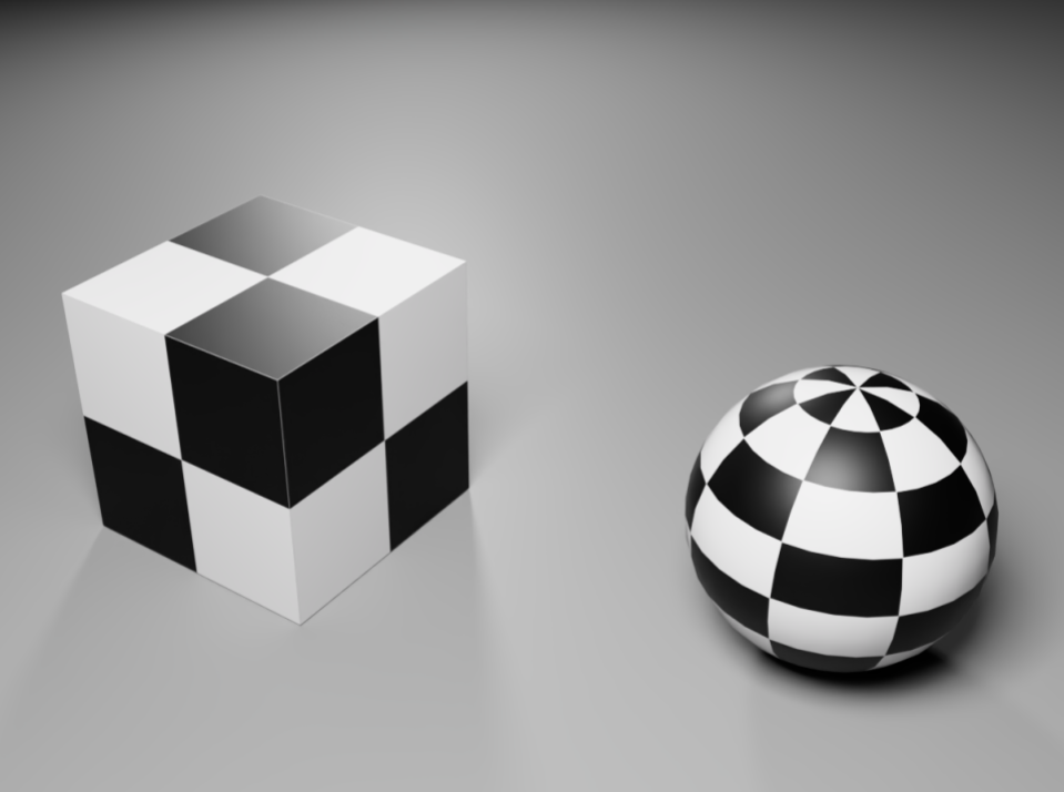
Figure 1:The ‘physics.usda’ stage showing the cube and sphere that we will use to demonstrate basic physics.
You should have the following directory structure for this physics simulation:
/Ch08
├── Assets
│   ├── textures
│   │   └── <All Texture Files>
│   ├── Cube.usd
│   └── Sphere.usd
├── physics.usda
└── swinging_sticks.usda
Remember to set ‘/Ch08’ as your working directory using:
import os

new_directory = <'/your/path/to/Ch08'>

os.chdir(new_directory)
Let’s dive straight into a physics simulation of a cube and ball interacting with each other and the ground beneath them. To achieve this, we’ll open the stage provided and add the elements necessary for a physics simulation to run, such as Rigid Bodies, Colliders, and Mass, then we’ll explore more subtle aspects of simulation that enhance the realism, such as friction, bounciness, and density.
This time we’re not going to create a new stage; we can simply open the existing ‘physics.usda’ stage that we’ve provided in the Ch07 directory. First let’s import the necessary modules, including UsdPhysics, then we can open the stage:
from pxr import Usd, UsdGeom, Gf, Sdf, UsdPhysics

# Define the path using a relative path as our working directory is set to '/Ch07'
usd_file_path = '<path/to/your/file.usd ex: "./physics.usda">'

# Open the 'physics.usda' stage
stage = Usd.Stage.Open(usd_file_path)
The stage contains a cube, a sphere and a ground plane. Shortly, we’ll want to use the path strings of their meshes to apply physics attributes to them. To easily access their path strings, let’s modify the stage.Traverse() method that we used in Chapter 2 to iterate over the stage and print the relevant path strings. This modification will allow us to print the path strings of only the mesh prims (ignoring lights and materials) by adding an if statement within the Traverse method to check if a prim is a mesh before printing its path string:
# Traverse the stage
for prim in stage.Traverse():
    # Check if the prim is a UsdGeom.Mesh and ignore other types of prim
    if UsdGeom.Mesh(prim):
        # Print pathStrings
        print(prim.GetPath().pathString)
All being well, the code snippet above should print the following path strings:
/World/GroundPlane/CollisionMesh
/World/Sphere/Sphere_mesh
/World/Cube/Cube_mesh
8.1.1 Computing Bounding Boxes
As we’re going to apply physics attributes to the cube and sphere, let’s add a bounding box to each of them. Remember from Chapter 5 that the bounding box is essential for calculating collisions because it defines the extent of an object using two points: the minimum and maximum corners of the object’s mesh. These points represent the overall volume that the object occupies in 3D space, making it possible to detect collisions with other objects based on their bounding boxes.
For efficiency, we’ll create a custom function before calling it on each object in turn. We can repeat the approach we used in Chapter 5, Listing 5.4:
# Define the function ‘compute_bounding_box’ for a specified prim in a given stage
def compute_bounding_box(stage, prim_path):
    prim = stage.GetPrimAtPath(prim_path)

    # Set the purpose of getting the bounding box, "default" for general purposes
    purposes = [UsdGeom.Tokens.default_]

    # Get the box cache
    bboxcache = UsdGeom.BBoxCache(Usd.TimeCode.Default(), purposes)

    # Compute the bounding box
    bboxes = bboxcache.ComputeWorldBound(prim)

    # Get the box vertices
    min_point = bboxes.ComputeAlignedRange().GetMin()
    max_point = bboxes.ComputeAlignedRange().GetMax()

    # Returns the computed min and max points of the bounding box
    return min_point, max_point
Having defined the ‘compute_bounding_box’ function, let’s call it on both the cube and sphere, then use the min/max points to set the Extent of the meshes. We can use a list of paths to call compute_bounding_box for multiple prims at once:
# List of prim paths for the sphere and cube
prim_paths = ['/World/Sphere/Sphere_mesh', '/World/Cube/Cube_mesh']

# Iterate over the list
for path in prim_paths:
    # Calls the custom function to compute the bounding box, returning the min and max points of the object's extent
    min_point, max_point = compute_bounding_box(stage, path)

    # Get the mesh prim
    mesh = UsdGeom.Mesh(stage.GetPrimAtPath(path))

    # Set the ExtentAttr for both meshes
    mesh.CreateExtentAttr([min_point, max_point])

stage.Save()
We’ve now established the extent of the cube and sphere, but we’ve yet to determine how they will behave in a physics simulation. For that, we’ll need to assign some physical properties to the meshes.
8.1.2 Applying Physical Properties
The UsdPhysics schema allows for many physical properties to be applied to objects. By defining the physical properties of an object, UsdPhysics can simulate the motion and interaction of rigid bodies in a realistic and accurate way. The first three physical properties we’re going to explore are:
- Body Type: Refers to the classification of an object in a physics simulation, indicating how it behaves in terms of motion and interaction with other objects.
- Collision Detection: Used to specify whether an object should participate in collision detection during simulations.
- Mass: Defines the mass of the object, which affects its response to forces like gravity and interactions with other objects.
Let’s apply each of these in turn to our cube and sphere.
Rigid and Deformable Body Types
There are two primary body types:
- Rigid Bodies: Objects that maintain a constant shape and volume during simulation. These bodies are modeled with fixed geometry, and their interactions, such as collisions, are governed by rigid body dynamics, meaning they don’t deform under forces. Common examples include solid objects made of metal, rocks or glass.
- Deformable Bodies: These are objects that can deform or change shape in response to forces. Unlike rigid bodies, soft bodies allow for simulations that model flexibility and stretching, such as cloth, flesh or jelly-like materials. This property is useful for more complex interactions where the object’s shape changes dynamically under forces. Deformable Bodies are currently best implemented using NVIDIA Omniverse’s native PhysX API rather than the OpenUSD framework. As this approach differs from the methods covered in this chapter, we’ve included a brief introduction to PhysX API basics in Appendix C.
Let’s add a rigid body to the cube and sphere using the RigidBodyAPI.Apply() method. As we’ve already created the ‘prim_paths’ list that contains both meshes, we can use that to apply the rigid body to both at the same time:
# Iterate over the list
for path in prim_paths:
    # Get the UsdPrim
    prim = stage.GetPrimAtPath(path)
    # Apply RigidBodyAPI
    UsdPhysics.RigidBodyAPI.Apply(prim)

stage.Save()
Now that the meshes have rigid bodies, they will respond to gravity when the physics simulation is run.
In USD Composer physics simulations are run in a slightly different way than animations. Where an animation will play through a set number of frames before looping back to the start, once running, a physics simulation will continue indefinitely until paused or stopped. In most simulations, objects eventually come to rest. To improve performance, rigid body simulation will ‘Sleep’ objects that have reached an equilibrium state, meaning that the object’s interactions are no longer calculated until it is disturbed in any way.
To run a simulation, there is a ‘Play’, ‘Pause’ and ‘Stop’ button available in the default Toolbar located at the far left of the UI (See Figure 2).
The Play button will start the simulation and cause a Pause and Stop button to appear in its place. The Pause button will halt the physics simulation at whatever point it has reached and the Stop button will halt the simulation returning the stage to its initial state.
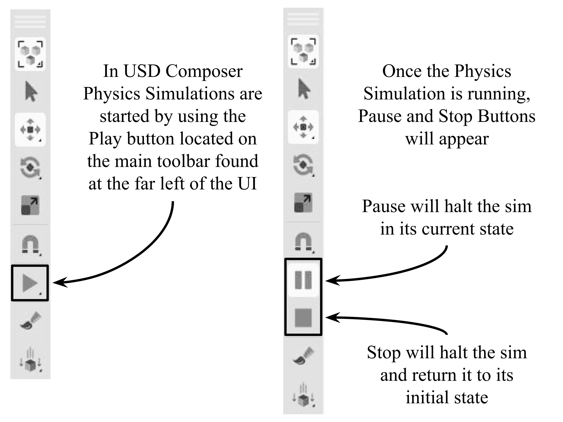
Figure 2:Located at the far left of the UI, USD Composer’s default Toolbar has Play, Pause & Stop buttons for running physics simulations.
If you press Play on our ‘physics.usda’ stage you will see the cube and sphere come under the effect of gravity, dropping away through the ground. You’ll notice that pressing pause only halts the simulation with the cube and sphere still located somewhere below the ground. If you press Play again, they will continue to fall from where they were when the simulation was paused. However, pressing Stop will halt the simulation and return everything to its initial state, returning the cube and sphere to their starting point above ground.
Obviously, having objects fall through the ground is generally undesirable. To avoid this, and to allow the objects to interact with each other, they need to be given a Collision Shape, also called a Collider.
Collision Detection
Giving an object a collider is essentially applying a constraint that will prevent it from passing through any other solid body that it meets. To provide more flexibility and control over simulations, OpenUSD made the rigid body and collider separate entities. One advantage of this is to make it possible to create Static Colliders, objects that will remain unaffected by any force, but still be calculated during collision detection such as a wall or a floor.
In our example scene, the GroundPlane already has a collider, but no rigid body. This makes it a static collider and prevents it from responding to gravity when the simulation is run. However, even though the GroundPlane already has a collider, it did not prevent the cube and sphere from falling through it. This is because they don’t yet have their own colliders, and only a collider will interact with another collider.
To prevent the cube and sphere from passing through the GroundPlane, let’s give them colliders by iterating over the same ‘prim_paths’ list that we used previously, and using the CollisionAPI.Apply() method:
# Iterate over the list
for path in prim_paths:
    # Get the UsdPrim
    prim = stage.GetPrimAtPath(path)
    # Apply CollisionAPI
    UsdPhysics.CollisionAPI.Apply(prim)

stage.Save()
Now when the simulation is started using the Play button, the cube and sphere will not fall through the ground as their colliders will interact with the existing ground collider.
Another neat feature of USD Composer is that it allows us to interact directly with the objects in a physics scene by grabbing them with the mouse and pulling them around to simulate forces acting on them. Figure 3 shows the cube being manipulated in this way. To try this out for yourself, once the simulation is started move the mouse over the cube, press shift on your keyboard and left mouse click, then move the mouse around to pull the cube. You will notice a small red circle appears to show you the point at which you have grabbed the cube, and a green line will extend from the point of contact in the direction that you move the mouse. The green line will extend in length according to how hard you are pulling.
If you’ve been playing with this, you will probably have flung the cube or sphere right out of the scene by now. Remember, you can return the scene to its original state by clicking the stop button.
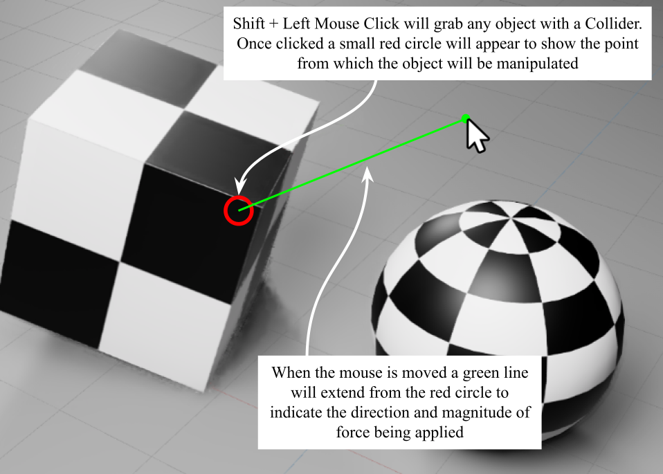
Figure 3:Physics manipulation in USD Composer. Once the simulation is started with the Play button any object with a Collider can be grabbed by positioning the mouse pointer over the object and using Shift + Left Mouse Click. Once grabbed, the mouse can be moved to simulate a pulling force acting on the object.
The ability to manipulate objects live in a simulation can be very useful for testing out your collider, observing how objects interact, or even for arranging objects in a scene in a very natural way.
If you tried moving the sphere while the simulation is running, you will notice that it didn’t move very realistically, but rolls as though it has lots of flat faces rather than a spherical surface. This happens because the collider is simply copying the shape of the mesh, and this sphere is ‘low poly’, meaning it has been made with very few faces.
To resolve this and make the sphere roll smoothly, we can adjust how the collider responds to the mesh. OpenUSD offers the MeshCollisionAPI, which provides finer control over the type of collider that is applied to a mesh.
Mesh Collision
The basic CollisionAPI is sufficient for identifying objects as colliders by adding the necessary metadata to the prim. However, it is common for USD stages to be populated with detailed models that are formed from complex meshes. Highly complex meshes can be computationally expensive during physics simulations, and very low poly meshes may not behave realistically as our sphere demonstrates. Therefore, UsdPhysics provides another type of API that addresses these issues, the MeshCollisionAPI.
Both the Collision API and the MeshCollision API can coexist on the same mesh. The MeshCollisionAPI extends the functionality of the Collision API, providing more control over how the collider behaves irrespective of the mesh it is applied to. It allows for customizable collision shapes tailored to the desired balance of accuracy and computational efficiency.
These customizable collision shapes are referred to as approximations as they approximate the mesh they are applied to, and they are assigned as an attribute named physics:approximation.
There are several types of approximation available:
- Bounding volumes: These are simple shapes, such as spheres, boxes, or capsules, that enclose the object. Collision detection is first performed on the bounding volumes, and only when they actually collide is a more detailed check performed on the actual geometry of the object.
- Convex hulls: These are convex shapes that enclose the object and touch all of its vertices. They are more accurate than bounding volumes but still simpler than the actual object geometry of a complex mesh.
- Simplified meshes: These are reduced-resolution versions of the object’s mesh, with fewer vertices and faces. They are less accurate than the original mesh but still provide a good approximation for collision detection.
The choice of approximation depends on the complexity of the object’s mesh, the desired accuracy of the simulation, and the available computational resources. For example, the model of a vehicle used in a game might have a very complex mesh making collision computation expensive. Giving the vehicle a simpler approximation of its mesh, such as a convex hull, or simplified mesh and using that to calculate collisions is much more efficient and more suited to gaming.
In contrast, approximations can also be used to make low poly meshes behave as though they were smoother. For example, in our cube and sphere simulation the sphere is not rolling smoothly because its low face count gives its collider lots of flat surfaces. To get the sphere moving realistically we can apply a bounding volume type of approximation that more closely resembles a smooth sphere. This is done by setting the physics:approximation attribute to ‘boundingSphere’.
The cube doesn’t need any additional approximation as it is behaving as expected with the basic CollisionAPI.
Let’s fix our sphere simulation by using the MeshCollisionAPI.Apply() method, then we can set the approximation type attribute to ‘boundingSphere’ with the GetApproximationAttr().Set method:
sphere_mesh_path = '/World/Sphere/Sphere_mesh'

# Get the prim at '/World/Sphere/Sphere_mesh'
sphere_prim = stage.GetPrimAtPath(sphere_mesh_path)

# Apply the MeshCollisionAPI to make the physics:approximation attribute available
mesh_collision_api = UsdPhysics.MeshCollisionAPI.Apply(sphere_prim)

# Set the physics:approximation attribute to "boundingSphere"
mesh_collision_api.GetApproximationAttr().Set("boundingSphere")

stage.Save()
Now when you run the simulation and manipulate the sphere you will see that it is rolling perfectly smoothly.
Mass
Another important physical property to consider is the mass of an object. Since the cube and sphere have had Rigid Bodies applied, their mass will be automatically computed based on the collision geometry and a default density. However, we can also define the mass of an object by calling the MassAPI.
First let’s add mass to the sphere by using the MassAPI.Apply() method and creating a Mass Attribute with CreatMassAttr():
# Apply MassAPI to the sphere_prim
mass_api = UsdPhysics.MassAPI.Apply(sphere_prim)

# Set mass
mass_api.CreateMassAttr().Set(10000.0)

stage.Save()
Now, if we run the physics simulation and roll the sphere so that it collides with the cube, the sphere will move the cube much more easily as it has a higher mass.
Next let’s add mass to the cube by first getting the prim, then applying the same method but giving the cube a much higher mass value:
cube_mesh_path = '/World/Cube/Cube_mesh'

# Get the prim at '/World/Cube/Cube_mesh'
cube_prim = stage.GetPrimAtPath(cube_mesh_path)

# Apply MassAPI to the cube_prim
mass_api = UsdPhysics.MassAPI.Apply(cube_prim)

# Set mass
mass_api.CreateMassAttr().Set(100000.0)

stage.Save()
Now when we roll the sphere into the cube, the cube moves much less due to the higher mass value of the cube.
Although the physics simulation is now looking realistic, you might have noticed that the objects are behaving as though they are sliding around on ice. This is because we have not added any friction to the surfaces yet. To do this, we need to start applying Physics Materials.
8.1.3 Defining Physics Materials
In OpenUSD Physics Materials are conceptually similar to visual materials, but instead of defining appearance, as demonstrated in Chapter 3, they specify physical behaviors during collisions or contact. Physics Materials do this by defining values for physical properties such as friction, bounciness, and density. These properties are applied using the UsdPhysicsMaterialAPI and can be shared across multiple objects.
A mesh prim can bind both the visual material and physics material at the same time. These can either be two separate materials, or the visual and physical properties can be combined into one material. For example, imagine a game that has lots of walls for the player to collide with and bounce off. If all of the walls are intended to look the same and be equally bouncy, then a combined physics and visual material can be used for all of them. If, however, you want some walls to have a different appearance but all walls to remain equally bouncy, then you would use different visual materials on each wall but the same physics material on all walls, necessitating the use of multiple separate materials.
Physics Material properties relate to attributes that define surface interactions as follows:
Static Friction: The resistance to initial motion between two surfaces in contact.
Dynamic Friction: The resistance to motion when two surfaces are sliding against each other.
Restitution: The bounciness of a collision, defined as the ratio of relative velocity after impact to that before impact.
Density: The mass per unit volume of a material, affecting how it behaves in simulations involving buoyancy or forces.
Figure 4 shows a graphic representation of situations where the two types of friction, and restitution may be required in a simulation.
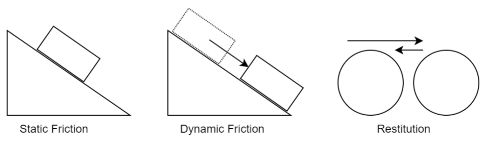
Figure 4:Illustration of physics materials properties. Static Friction is the resistance to the initial movement between two surfaces in contact; Dynamic Friction is the resistance encountered between two moving surfaces; Restitution measures the bounciness of a collision, determining how much kinetic energy is conserved or lost when objects collide.
The attribute ranges for static friction, dynamic friction, and restitution are typically determined by the physics simulation engine being used (e.g., NVIDIA PhysX). While OpenUSD itself doesn’t enforce strict limits on these attributes, Table 1 shows the general guidelines based on standard physics engines:
Table 1 Guidelines on Attribute Ranges for Physics Properties
Table 1:Physics Properties: Typical Ranges, Common Usage, and Notes.
| Property Name | Typical Range | Common Usage | Notes |
|---|---|---|---|
| Static Friction (StaticFrictionAttr) | 0.0 to | 0.0: Perfectly slippery surface 1.0: Typical realistic friction for common surfaces Values > 1.0: High-friction surfaces like rubber on asphalt | Some physics engines may clamp this value to reasonable limits internally, even though theoretically no upper limit exists. |
| Dynamic Friction (DynamicFrictionAttr) | 0.0 to | 0.0: No resistance to sliding 0.1–1.0: Realistic range for most materials Values > 1.0: High-friction scenarios | Dynamic friction is usually less than or equal to static friction for stability in simulations. |
| Restitution (RestitutionAttr) | 0.0 to 1.0 | 0.0: Perfectly inelastic collisions (no bounce) 1.0: Perfectly elastic collisions (full bounce without energy loss) | Values outside this range are not physically meaningful and may cause undefined behavior. |
Let’s begin adding a physics material to our sphere.
There is a ‘quick and dirty’ way to do this by binding the physics material directly to a prim using UsdPhysics.MaterialAPI.Apply(prim). We’re not going to do it that way, because whilst this is fine in some situations like quick test simulations, it can cause problems if the material later needs to be removed from an object that also has visual material bindings, and it makes the material harder to find in a complex stage hierarchy. It is better practice to use a less direct, more flexible approach by creating a physics material as a standalone prim. Like a visual material, this acts as a container for material properties, can be easily found in the hierarchy, and be bound to multiple prims.
Just as we did in Chapter 4 when creating visual materials, we’ll need to import the UsdShade module and use it to create a physics material as a discrete prim. After defining the physics material we can apply the PhysicsMaterialAPI schema to the material prim. This allows us to create and set the physics-specific attributes that will be contained by the physics material prim:
from pxr import UsdShade

# Define Physics Material using UsdShade module
physics_material = UsdShade.Material.Define(stage, "/World/PhysicsMaterial")

# Apply the PhysicsMaterialAPI schema to the material prim to define physics-specific attributes
physics_material_api = UsdPhysics.MaterialAPI.Apply(physics_material.GetPrim())
# Create StaticFriction attribute and set it to a relatively high level
physics_material_api.CreateStaticFrictionAttr().Set(0.9)

# Create DynamicFriction attribute and set it to a value slightly below the StaticFriction value
physics_material_api.CreateDynamicFrictionAttr().Set(0.8)

# Create Restitution attribute
physics_material_api.CreateRestitutionAttr().Set(1.0)
stage.Save()
Note We could also set the Density value of the physics material using physics_material_api.CreateDensityAttr().Set(). However, we don’t need to do this in this example as we have already set the Mass of the cube and sphere. We’ll discuss the relationship between mass and density shortly, under ‘Setting Density’.
If you now view the stage hierarchy in USD Composer, you will see the Physics Material prim, and selecting it will show the properties tab below which displays the values of each attribute. (See Figure 5)
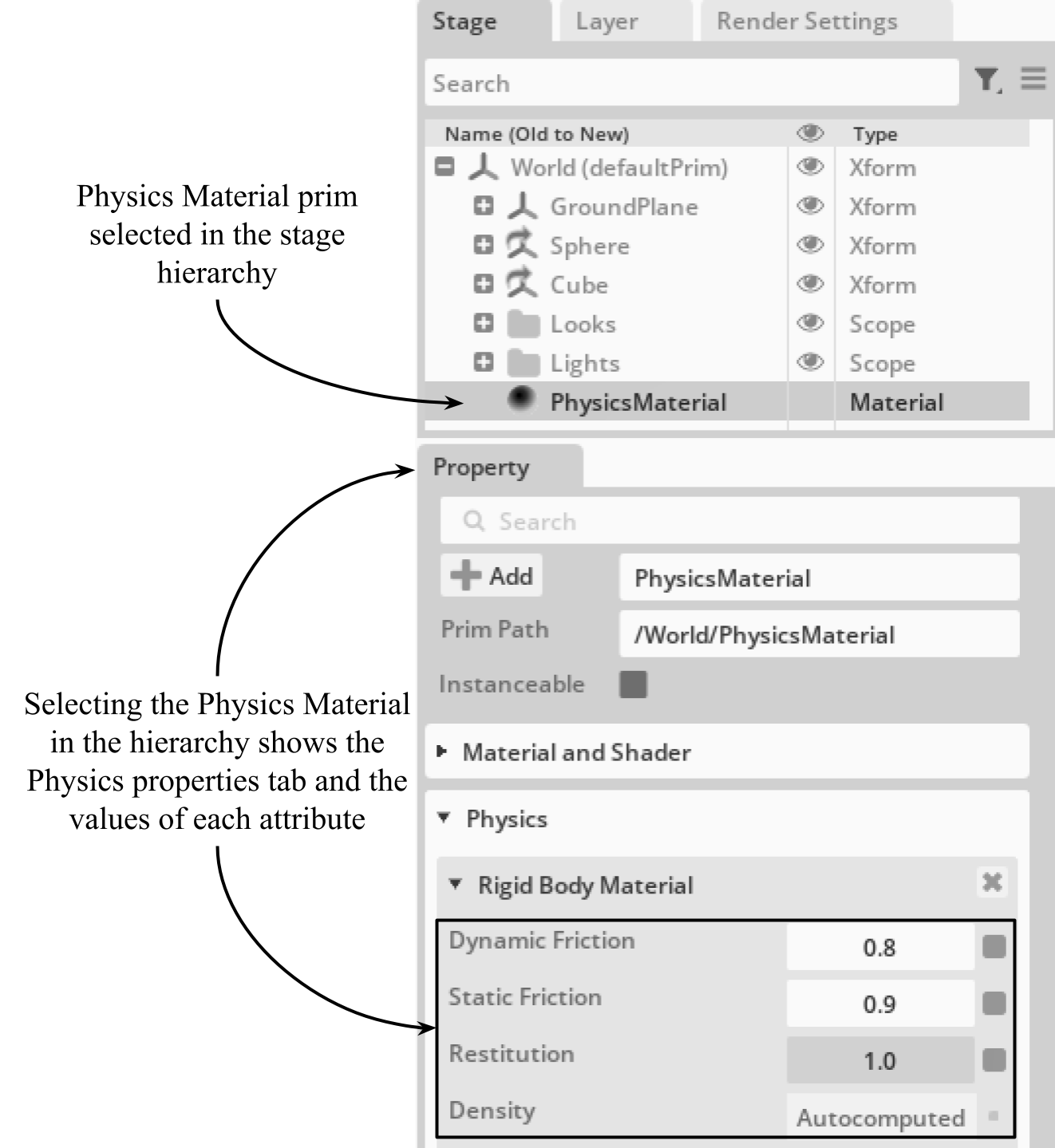
Figure 5:The newly created Physics Material shows up in the hierarchy of the stage in USD Composer. Clicking on the Physics Material will show the properties tab below, which shows the values of each attribute.
At present the physics material has not been applied to any objects on the stage. Let’s go ahead and bind it to the sphere. We’ll combine the CreateRelationship() method, and the AddTarget() method to bind the physics material to the sphere prim:
# Get the sphere_prim
sphere_prim = stage.GetPrimAtPath("/World/Sphere/Sphere_mesh")        #A

# Create the material binding relationship and apply the Physics Material to the sphere_prim
sphere_prim.CreateRelationship("material:binding:physics").AddTarget(physics_material.GetPath())    #B

stage.Save()
Now if we run the simulation in USD Composer the sphere will be much more bouncy like a hard plastic ball.
If we use the same approach to add the physics material to our cube we can make that equally bouncy:
# Get the prim for the cube
cube_prim = stage.GetPrimAtPath("/World/Cube/Cube_mesh")    #A

# Create the material binding relationship and apply the Physics Material to the cube_prim
cube_prim.CreateRelationship("material:binding:physics").AddTarget(physics_material.GetPath())    #B

stage.Save()
Running the simulation now and dragging the cube around at ground level, we can clearly see the effects of the higher friction values making the cube slide around less as it drags across the ground.
Now that the physical attributes have been created, we can easily edit their values. For example, if we wanted the physics material to be more slippery and less bouncy, we would Get each attribute and use the Set() method as follows:
# Get StaticFriction attribute and set it to a relatively low level
physics_material_api.GetStaticFrictionAttr().Set(0.1)    #A

# Get DynamicFriction attribute and set it to a value below the StaticFriction value
physics_material_api.GetDynamicFrictionAttr().Set(0.05)    #B

# Get Restitution attribute and set it to low bounciness
physics_material_api.GetRestitutionAttr().Set(0.1)    #C

stage.Save()
It’s important to note that in real-world physics, friction and restitution are properties of the interaction between two surfaces rather than an inherent property of a single material. PhysX approximates this by assigning friction and restitution coefficients to individual materials and combining them during interactions. The method of combining these coefficients can significantly affect the simulation’s realism, and selecting the best method can make the simulation of specific materials much more accurate. PhysX offers different combine modes to determine how the friction and restitution values of two colliding materials are combined. The combine mode options are average, min, max, and multiply, represented as tokens in OpenUSD. (Tokens are a lightweight, string-like data type used for enumerations in attributes.)
When a physics material is created the combination mode for both friction and restitution will default to average. Each combination mode calculates the coefficient as follows:
- Average: Takes the mean of the two values
- Min: Uses the smaller of the two values
- Max: Uses the larger of the two values
- Multiply: Multiplies the two values together
We could leave our physics material in the default ‘average’ combination mode as the results are looking realistic. However, there may be times when you are simulating a very specific material where altering the combination mode might get the results you are after. Due to the complexity and variability of real-world interactions, it’s common practice to adjust the values and combination modes of friction and restitution experimentally within the simulation to achieve the desired behavior.
Setting the combination mode can be done using similar methods to those we used above to set the PhysicsMaterial properties. However, the CreateAttribute() method is not available on the MaterialAPI class directly, as it’s meant for creating attributes on the Prim object itself. So, in this case we’ll use the GetPrim() method to create the attribute on the physics_material prim. Also, for maximum fun with our bouncing sphere, let’s set the restitution back to a high value, as follows:
# Change the restitution back to 1.0 for lots of bounciness
physics_material_api.GetRestitutionAttr().Set(1.0)    #A

# Set the restitution combine mode to 'max' on the physics_material prim
physics_material.GetPrim().CreateAttribute("physxMaterial:restitutionCombineMode", Sdf.ValueTypeNames.Token).Set("max")    #B

# Set the friction combine mode to 'min' on the physics_material prim
physics_material.GetPrim().CreateAttribute("physxMaterial:frictionCombineMode", Sdf.ValueTypeNames.Token).Set("min")    #C

stage.Save()
As the material is already bound to the objects, they will now behave differently when the simulation is run. Notice how the sphere is now even more bouncy than it was when we had the restitution at its full value and the combination mode defaulting to average. Now it’s more like a rubber ball than a hard plastic ball because the restitution is only being calculated with the maximum value of the two materials that are interacting. Therefore, when it collides with the ground, it ignores the less bouncy ground. Also notice that though the friction was already relatively low, setting the combination method to minimum has allowed the cube to slide around a bit more.
In summary, by carefully setting the static and dynamic friction coefficients, restitution values, and selecting suitable combine modes, you can simulate a wide range of material behaviors in PhysX. Due to the lack of standardized property values for specific materials, iterative testing and adjustment within your simulation environment are recommended to achieve realistic results.
Setting Density
Setting the density using the UsdPhysicsMaterialAPI does not directly override a mass attribute already set on an object. Instead, it influences how the mass is calculated if the mass is not explicitly defined. The physics engine will behave as follows:
- If mass is explicitly defined on the object, that value takes precedence, and the density will not affect it.
- If mass is not explicitly set, the physics engine will compute the mass based on the object’s volume and the specified density.
This allows for flexibility:
- Use mass for direct control over an object’s weight.
- Use density for dynamically computed mass based on the object’s geometry.
Avoid setting both mass and density unless you intentionally want mass to take precedence. In such cases, density will have no effect on the object’s mass calculation.
The physics properties that we’ve been working with so far can be thought of as Constraints. In other words, we have been putting limitations on objects using things like colliders to prevent them passing through other objects, or material properties that enforce a particular type of behaviour. Everything we’ve done so far can be thought of as adding ‘Implicit Constraints’.
In the next section we will begin dealing with ‘Explicit Constraints’. These take the form of fixed spatial relationships between two objects, such as the limitation that one object can only rotate on one axis relative to another object like a hinge, or perhaps one object will only slide along one axis relative to another object like a piston. These types of explicit constraints are usually referred to as joints.
8.2 Combining Multiple Parts with Joints
In the real world, complex objects are often composed of multiple parts that are connected together to form a single, functional whole. In OpenUSD, you can replicate this complexity by combining multiple rigid bodies with joints, which define the relationships between the parts and constrain their relative motion. We can use the UsdPhysicsJoint prim for creating these connections to build articulated objects that can be simulated and animated in a physically realistic way.
We will demonstrate the application of joints with a simple two jointed structure, but the same principle can be used to create a wide range of more complex objects, from robots and machinery to characters and creatures.
The number of independent ways in which a joint can move is measured in ‘Degrees of Freedom’ (DOF). Any object in 3D space can have up to 6 degrees of freedom: 3 for translation and 3 for rotation. Each joint type constrains the movement of a prim within its possible mode of translation or rotation, with the exception of the D6 joint which is designed to use all 6 DOF.
Joints can be used to fix two objects together in a static way with a fixed joint which allows 0 DOF, or to model flexible connections such as hinges, ball joints or sliding structures which have 1 or more DOF.
The four commonly used joint types provide the following behaviours:
- Fixed Joint: A fixed joint rigidly connects two bodies, preventing any relative motion between them. This joint is useful for aggregating multiple bodies into a single, rigid unit. Example: Two welded metal beams.
- Prismatic Joint: A prismatic joint allows motion along a single axis, while preventing rotation and motion in all other directions. Example: pistons, drawers, sliding doors and windows.
- Revolute Joint: A revolute joint allows rotation around a single axis, while preventing motion in all other directions. Example: hinges and axles.
- D6 Joint: A D6 joint is a general-purpose joint that allows motion in all six degrees of freedom. This joint can be used to model complex connections and can also be constrained to limit motion in specific directions using less than 6 DOF if required.
Figure 6 shows four commonly used joint types.
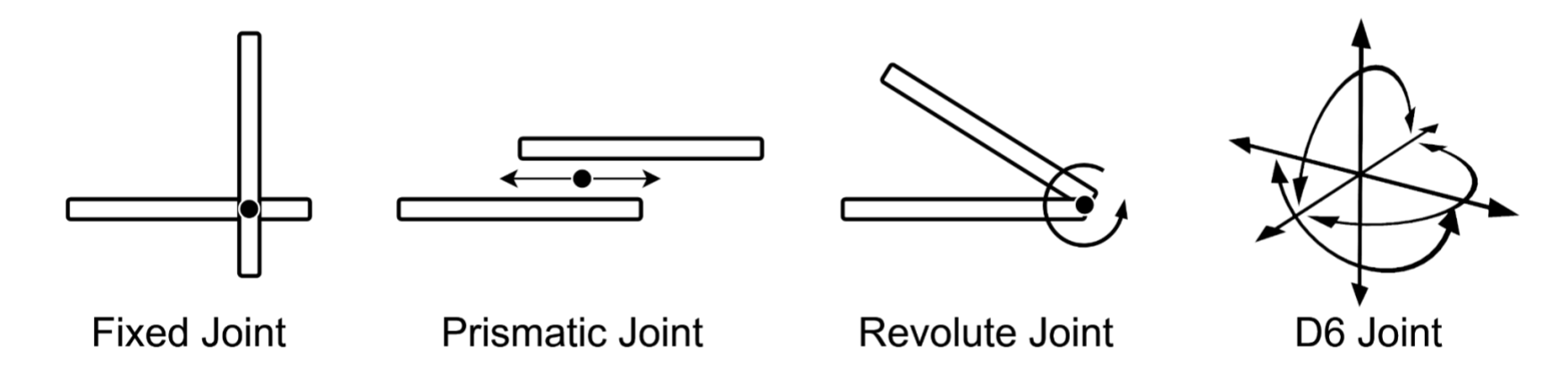
Figure 6:Four Commonly Used UsdPhysicsJoint Types.
Table 2 gives a comparison of these joint types including their API name, DOF and function.
Table 2:Comparison between UsdPhysics Joint Types.
| Joint Name | API Name | Dof | Function |
|---|---|---|---|
| Fixed Joint | UsdPhysics.FixedJoint | 0 | Fix one body on another |
| Prismatic Joint | UsdPhysics.PrismaticJoint | 1 | Slide one body from another |
| Revolute Joint | UsdPhysics.RevoluteJoint | 1 | Rotate one body from another |
| D6 Joint | UsdPhysics.Joint | 6 | Joint for general purposes |
Let’s learn how to apply joints by building a model of the Swinging Sticks—a classic physics demonstration that showcases principles like conservation of momentum and energy. It simulates a double pendulum, also known as a chaotic pendulum in physics and mathematics as it simulates unpredictable movements. This kinetic sculpture, with its swinging parts, perfectly illustrates how to use revolute joints.
We have prepared a model specifically adding joints to the swinging sticks. If you haven’t already done so, remember to set ‘Ch08’ as your working directory using.
Figure 7 illustrates the types and positions of the joints required to capture the dynamics of the swinging sticks: the first stick is configured to rotate around the top of the supporting base, while the second stick is set up to rotate around the end of the first stick. These joint configurations are essential for accurately simulating the physical interactions and swinging motion of the sticks.
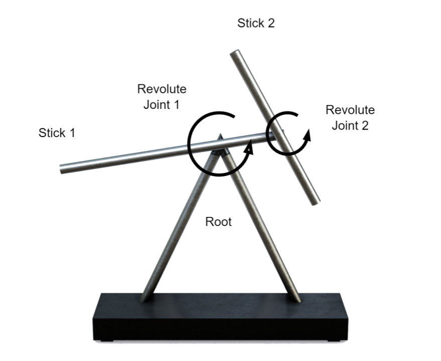
Figure 7:A Screenshot of the Swinging Sticks model. It consists of the base support, and two sticks each of which has a joint to rotate around. The whole system simulates a double pendulum, also known as a chaotic pendulum as it simulates unpredictable movements.
First, let’s open the downloaded stage:
from pxr import Usd, UsdGeom, Gf, UsdPhysics

# Define the path using a relative path as our working directory is set to '/Ch07'
usd_file_path = <'path/to/your/file.usd' ex: './swinging_sticks.usda'>    #A
stage = Usd.Stage.Open(usd_file_path)    #B
Note On this stage we have set the ‘z’ axis as the up axis instead of the ‘y’ up that we have used on previous stages. This is so that you can get used to working with different up axes, as some projects will require a specific up axis and ‘z’ or ‘y’ are both commonly used.
Currently, there are no joints in the stage and you can only see the raw model: the base, two sticks, and a support which will provide a fulcrum from which one of the sticks will swing. Before adding the joints, let’s make sure that the two sticks have RigidBody APIs since joints always work together with rigid bodies in OpenUSD. We can also add Colliders so that we can use the shift/click method of interacting with the sticks when the simulation is running, just as we did with the cube and sphere earlier.
Let’s use a list of prims again to make the application of rigid bodies and colliders as efficient as possible:
# Create a list of the stick prims
prim_paths = ['/root/swing/stick1', '/root/swing/stick2']

# Iterate over the list
for path in prim_paths:
    # Get the prims at the specified paths
    sticks = stage.GetPrimAtPath(path)

    # Apply rigid bodies to all prims in the list
    UsdPhysics.RigidBodyAPI.Apply(sticks)

    # Apply colliders to all prims in the list
    UsdPhysics.CollisionAPI.Apply(sticks)
To function, any joint needs to be assigned two bodies that it will articulate. For example, the hinge of a door is a point of articulation between a door frame and a door. The object from which the joint’s movement originates is called ‘Body0’, and the object that moves in relation to Body0 is called ‘Body1’. In our example of a door, the door frame would be Body0 with the hinges attached to it, and the door itself would be Body1, which moves in relation to the door frame.
The revolute joint type allows an object to rotate around a single axis, so it is perfect for our swinging sticks model. Let’s add a joint using UsdPhysics.RevoluteJoint.Define(), to make the first stick rotate around the ‘support_fulcrum’ prim. In the following snippet we’ll create a relationship for Body0 and make it target the support_fulcrum using the CreateBody0Rel().SetTargets() method. We can then repeat this for Body1 which will target stick1. Finally, remembering that this stage has been set to use z as its up axis, we’ll define the revolute joint’s rotation axis as y by creating an axis attribute with CreateAxisAttr():
# Create a revolute joint as a child of the stick1 prim
revolute_joint1 = UsdPhysics.RevoluteJoint.Define(stage, "/root/swing/stick1/joint1")

# Set the target for Body0 to the support fulcrum
revolute_joint1.CreateBody0Rel().SetTargets(["/root/swing/support_fulcrum"])

# Set the target for Body1 to stick1
revolute_joint1.CreateBody1Rel().SetTargets(["/root/swing/stick1"])

# Set the rotation axis of the joint to the Y axis
revolute_joint1.CreateAxisAttr(UsdGeom.Tokens.y)

stage.Save()
If we now view the stage in USD Composer and run the simulation, we’ll see stick1 rotating around the y axis centered on the support_fulcrum. However, stick2 will simply fall away as it has yet to be joined to stick1 with another joint.
If we select the joint1 prim in the stage hierarchy, we can see in the viewport[d][e] that it has been positioned at the origin of the support_fulcrum as expected (See Figure 8 below). However, there are times when we might need to offset the position of a joint from the Body0’s origin. This swinging sticks model is a good example: to work properly, stick2 needs to rotate around the end of stick1, but stick1’s origin is at its center. Therefore, when we create a second revolute joint and set stick1 as its Body0 target it will be positioned at stick1’s origin near to its center instead of at its end. Figure 8 shows the position of joint1 at the support_fulcrum after we made it the target of joint1’s Body0. It also shows the position we are going to set for joint2 at the end of stick1, rather than at its center. Let’s explore a little more about how joints are positioned in OpenUSD.
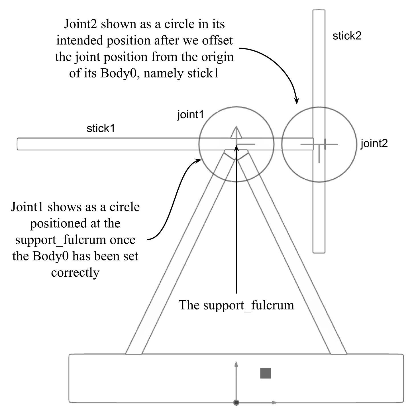
Figure 8:Showing the position of joint1 after the support_fulcrum has been set as the target for its Body0, and the position we intend to place joint2 at the end of stick one. This will be achieved by offsetting the local position of joint2 in relation to its Body0 at the origin of stick1.
When we first create the joint, it will be positioned at the World Origin. Once bodies have been assigned, the position of a joint is determined by its relative positioning to the two bodies it connects, Body0 and Body1. The joint itself has two primary attributes that define its local position with respect to each body:
- physics:localPos0: Defines the joint’s position relative to Body0 in its local coordinate space.
- physics:localPos1: Defines the joint’s position relative to Body1 in its local coordinate space.
By default, if the physics:localPos0 and physics:localPos1 attributes are not explicitly set, the joint’s position is assumed to align with the origins of the connected bodies. In this case, the joint will be positioned at the origin of the prim set as Body0, unless further adjustments are made, i.e., (Gf.Vec3f(0, 0, 0)).
To position a joint correctly in relation to both connected bodies, we need to explicitly set the physics:localPos0 and/or physics:localPos1 attributes. These attributes allow for precise control over where the joint is located relative to each body, ensuring proper alignment and behavior during simulation, especially when the bodies are moving or rotating.
To set the second joint in the correct position let’s offset it to the end of stick1. In the following snippet, we’ll set the Body0 and Body1 targets as we did for stick1, then we’ll get the physics:localPos0 attribute of the joint and adjust it using the GetAttrribute().Set() method:
# Create another revolute joint
revolute_joint2 = UsdPhysics.RevoluteJoint.Define(stage, "/root/swing/stick2/joint2")

# Set the target for Body0 to stick1
revolute_joint2.CreateBody0Rel().SetTargets(["/root/swing/stick1"])

# Set the target for Body1 to stick2
revolute_joint2.CreateBody1Rel().SetTargets(["/root/swing/stick2"])

# Set the rotation axis of the joint to the Y axis
revolute_joint2.CreateAxisAttr(UsdGeom.Tokens.y)

# Retrieve the prim from the revolute joint
joint2_prim = revolute_joint2.GetPrim()

# Set the translation
joint2_prim.GetAttribute("physics:localPos0").Set(Gf.Vec3d(0.038, -1.823, 0.54)[f][g])

stage.Save()
By creating the swinging sticks simulation, we have learned how to create joints, assign target bodies, and configure joint properties and positions. Now have some fun by running the simulation in USD Composer and using the shift/click method of grabbing the sticks and applying forces to make them swing around randomly.
Figure 9 showcases the dynamic behavior of the swinging sticks, highlighting how physics simulation can replace traditional animation techniques, offering a more accurate and efficient way to visualize movement. By leveraging Omniverse’s real-time feedback, you can iterate and refine physical interactions on the fly, making it an invaluable tool for both creative experimentation and precise scientific visualization.
Figure 9:Physics-Driven Animation of the Swinging Sticks in Omniverse. The animation of the swinging sticks is physics-driven instead of key-framed.
8.3 Articulations and Robots
In this section, we’ll briefly introduce articulations and robots, explaining the fundamental concepts and principles that govern their design and functionality.
In 3D simulation, an articulation refers to the joint or connection between two or more objects that allows for movement and flexibility in the body. In the context of robotics, articulation can also refer to multiple joints that work together to enable a specific range of motion. For instance, in the human arm, the articulation consists of multiple joints, the shoulder, elbow, and wrist, collectively allowing for a wide range of movements, from simple flexion and extension, to complex actions like rotation and circumduction.
In robotics, articulations function similarly, forming a series of joints that connect rigid components to enable motion and dexterity. Robotic joints are often designed to mimic human functionality, allowing robots to perform tasks such as grasping objects, locomotion, or interacting with their environment. By combining joints into articulated systems, robots can achieve complex movements that single rigid structures cannot perform. Figure 10 shows that although each individual joint may have limited DOF, the combination of joints can provide much greater range of movement.
The demonstrations we’ve given in this chapter provide you with everything you need to build a robot model with rigid bodies and colliders on its meshes, and joints applied between components to provide the desired articulation. Feel free to experiment and see what you can create.
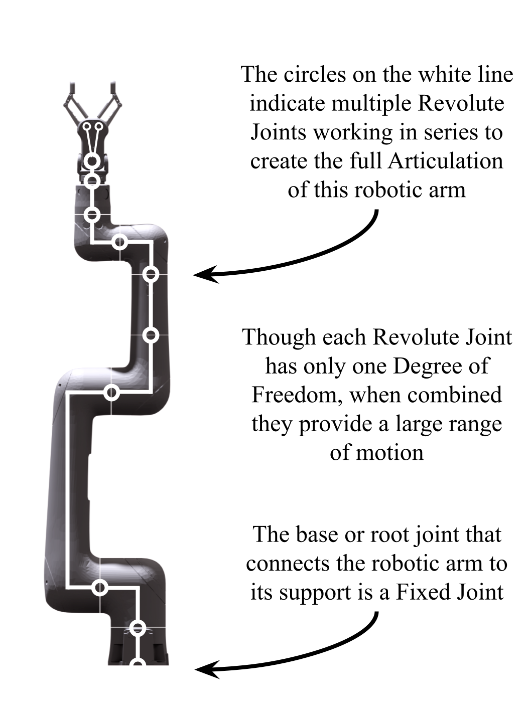
Figure 10:A robot represented as an articulation. It is composed of a chain of interconnected meshes and joints, illustrating how individual components work together to enable complex movements and large ranges of movement despite the single DOF of each individual joint.
Understanding articulations is essential for robotics, as it provides engineers with the tools to design systems capable of interacting with and adapting to their surroundings in more human-like ways. Insights from human anatomy and motion directly influence the development of robotic articulations, enabling innovations that enhance both fields. Advanced robotic systems, in turn, can contribute to a deeper understanding of biomechanics, fostering progress in areas such as prosthetics, rehabilitation, and human movement analysis.
Summary
- To see physical interactions in action, you must use a physics engine. This chapter demonstrated using NVIDIA Omniverse’s integrated physics engine, which seamlessly simulates UsdPhysics properties, offering real-time feedback and enhancing the realism of your scenes.
- UsdPhysics, a schema within OpenUSD, allows for defining physical properties like mass, collisions, and rigid body dynamics, enabling realistic simulations of objects in 3D environments.
- Physics materials, including properties like static friction, dynamic friction, and restitution, control how objects behave when interacting with each other, adding another layer of realism to your simulations.
- Various joints (like revolute, prismatic, and D6 joints) can connect rigid bodies, enabling complex articulated structures such as robotic arms and swinging pendulums.
- Joints must be assigned bodies from and on which to act, but their position can be changed in relation to those bodies by setting the local position accordingly.