This chapter covers
- Setting up animation on the stage
- Playing with Xform and property animation
- Composing animation clips

We have learned how to create a stage, populate it with objects, beautify it with materials and lighting, and make use of cameras to capture our creations. These skills are ample if we only wish to create static images from our scenes, but what if we want to set the scene in motion?
First we need to introduce the fourth dimension of time by applying a timeline to our stage. OpenUSD provides us with all the necessary tools through its UsdStage and UsdTimeCode classes which build on traditional time-based media concepts, allowing for additional flexibility across different platforms. We’ll examine this essential aspect of animation and see how it sets the stage for dynamic motion.
Once we have our timeline in place, we can start defining the movement and transformation of objects, lights, and cameras. By assigning values to properties at specific moments in time, we create keyframes that control the timing and extent of the animation. We’ll also explore how to smooth out our animations, using interpolation to fill in the frames between keyframes.
Finally, we’ll bring everything that we’ve learned together and create a new stage containing a model of a desktop fan. We’ll animate the fan blades to rotate and oscillate, and we’ll animate a camera move to demonstrate how changing viewpoints can add interest to a scene. By the end of this chapter, you’ll have a solid understanding of how to animate various elements of your scene, bringing life and movement to your OpenUSD projects.
But before we start animating, let’s first set up the stage properties to lay the groundwork.
7.1 Setting Up Stage Properties
Stage properties serve as the backbone of your animations, allowing you to control the global animation parameters that dictate how your scenes will behave in motion. Setting them correctly may also be necessary if your animation is intended to form part of a larger project which has predefined timecode requirements. For example, if you are creating an animation that will be used for a three second shot in a movie, you will need to match the movie’s framerate, measured in frames per second (fps). Once you know the fps, you can determine the number of frames you will need to create a three second animation. Most movies run at 24fps, so in this example 72 frames will give you three seconds worth of animation (24x3=72).
In a 3-second shot with 72 frames, the animation starts at frame 0 and ends at frame 71, following OpenUSD’s zero-based indexing—where counting begins at 0 rather than 1, as is common in programming and technical contexts.
All events in an animation can be thought of as happening on a timeline, and the point at which they occur on that timeline is given as a timecode. The timeline serves as a tool that organizes when and how different elements in a scene move or change over time, allowing animators to control the pacing and synchronization of events within the animation. Let’s begin by grasping the way OpenUSD approaches timecodes and how we can use methods from the UsdStage class to set up the stage properties ready for animation.
7.1.1 Understanding Timecode
In traditional film, video and animation media timecodes are defined by an agreed standard system called SMPTE (after the Society of Motion Picture and Television Engineers) which labels each frame by hours, minutes, seconds, and frames, synchronizing media assets to real-world time and playback speed. However, this strict structure can be limiting when different applications and industries have varying needs and ways of encoding time.
OpenUSD’s goal is to be highly flexible and broadly applicable across diverse workflows and software. Using SMPTE timecodes would require every application to conform to the same frame rate and unit system, which isn’t practical in the multiple environments that OpenUSD caters for. The ‘UsdStage’ class facilitates this flexibility by allowing both the framerate and number of time code units per second to be set independently.
Frames Per Second
The Fps value indicates the number of frames displayed per second of animation at the output or rendering stage, directly influencing the smoothness, pace of the motion and playback speed. It is defined on the stage using the stage.SetFramesPerSecond() method. If you are working on a pre-existing stage and need to know the fps you can use the stage.GetFramesPerSecond() method. Fps can be thought of as the playback resolution.
Time Codes Per Second
The Time codes per second value indicates the number of samples of time that are taken per second of animation. It does not determine the output rate, only the calculation rate when performing animations or simulations. It is defined on the stage using the ‘stage.SetTimeCodesPerSecond()’ method. If you are working on a pre-existing stage and need to know the time codes per second you can use the ‘stage.GetTimeCodesPerSecond()’ method. Time codes per second can be thought of as the temporal resolution.
The result of separating the output fps from the time codes per second is to allow for increased granularity in the way time is applied to the stage. This is useful in visual effects (VFX), scientific simulations, or when synchronizing different media sources when you may want to have more granular control over time. Let’s say you are creating a complex VFX animation where accuracy demands that physical simulations (such as cloth, fluids, or particle systems) need to be calculated at a higher temporal resolution than the visual output. You might want to perform calculations every 1/240th of a second (i.e., setting the TimeCodesPerSecond to 240) but only display frames at 30 Fps to match your intended output medium.
Another benefit of decoupling fps from time codes per second is to allow for greater interoperability across multiple platforms, especially when dealing with different software tools, hardware systems, or media formats that may have varying expectations for time representation. For example, if you need to convert or map animations across platforms with different frame rates (e.g., from 24 FPS to 30 FPS), adjusting TimeCodesPerSecond() separately allows for a more seamless conversion process, especially if you’ve set a higher-fidelity timecode information. This ensures that the animation maintains its timing accuracy even after being converted to a different frame rate.
OpenUSD’s UsdTimeCode Class
The UsdTimeCode class holds generic, unitless time values, allowing it to serve as an abstraction layer for time representation. The actual meaning of these time values—such as seconds or frames—is determined by the UsdStage, which references metadata in the file’s root to map the time to the appropriate units. This design offers several key benefits:
Unitless Flexibility: It allows each application to interpret time according to its needs, whether in seconds, frames, or other units, without enforcing a fixed time structure or frame rate.
Interchange Compatibility: By remaining unitless, USD files can easily transfer between different software and platforms with varying time standards, enabling seamless data sharing across studios, artists, and applications without the need for frame rate synchronization.
Future-Proofing: Since USD isn’t tied to a specific time format, it can adapt to future changes in time encoding, accommodating evolving time scales, resolutions, or playback standards.
This approach keeps USD versatile and adaptable, allowing it to accurately capture and translate between time systems in different environments while preserving the animator or designer’s intent.
In summary, A UsdTimeCode is just a way of representing time without specifying what “time” actually means (like seconds or frames). It’s like a placeholder or marker for time in USD files. When you work with a UsdStage, it helps to convert this generic time into something more specific, like seconds or frames. The UsdStage looks at metadata in the root layer of the file to figure out how to do this conversion.
This is a deeper understanding of timecode than we’ll need for our animations in this chapter, but well worth understanding for future applications of the knowledge you gain here. Next we’ll start setting some of that metadata on a new stage, preparing it for adding animation to some objects later on.
7.1.2 Setting the Stage’s Metadata
Start time, End time, Time Codes Per Second, and fps are fundamental parameters in a timeline that define the temporal structure of your sequence. Together, these settings control the timing and flow of your animation, ensuring that it plays out as intended within the defined time frame. Figure 1 shows an example of a timeline.

Figure 1:An example timeline. A timeline in the context of animation is a sequence that defines the duration and rate of frame progression in an animation, typically marked by a start time, end time, and frame rate (fps).
Let’s create a new stage and set it up ready to play with animations, remembering to ensure we are operating in the desired working directory for Ch07. This time we’re going to use the .usda format:
from pxr import Usd, UsdGeom, Gf, Sdf

stage = Usd.Stage.CreateNew("animation.usda")
For the purposes of demonstrating simple animation techniques, we don’t need to complicate things with separate fps and Time Codes Per Second values. To keep things straightforward, let’s first set the fps, and then synchronize the Time Codes Per Second by using stage.SetTimeCodesPerSecond(fps).
Then, we’ll use the SetStartTimeCode() and SetEndTimeCode() methods to start the timeline at frame 0 and stop at frame 59. The result will be an animation clip with a duration of 2 seconds (60 frames divided by 30 frames per second equals 2 seconds):
fps = 30.0

# Set fps
stage.SetTimeCodesPerSecond(fps)

# Set start time
stage.SetStartTimeCode(0)

# Set end time
stage.SetEndTimeCode(59)

stage.Save()
Accessing the Timeline in Your Viewer
With the stage created and the global animation parameters set, let’s learn how to access the timeline in your chosen viewer. Figure 2 shows the timeline as it appears in each of the viewers. Each timeline will show both the start and end frame number, and will have a play button to trigger the animation in the viewport. Once triggered, the animation will play through to the end frame then cycle back to the start and repeat until stopped.

Figure 2:The Timeline in USDView, Blender and USD Composer. Each viewer will show the start frame, end frame, and Play button.
USDView will have the timeline visible on launch. It is located at the bottom of the screen.
Blender will also have the timeline visible on launch, provided you are in the Layout tab. If for any reason the timeline is not visible, it can be opened using the button at the top left of any window which opens a menu that lets you select the Editor Type. (See Figure 3)
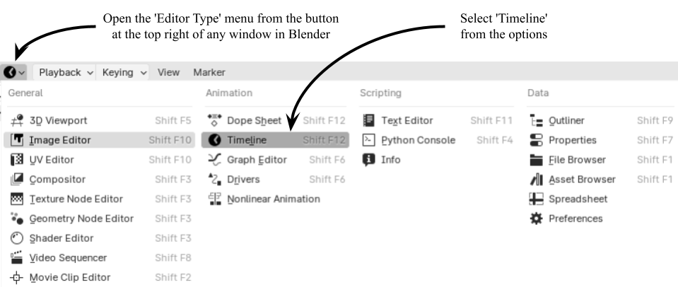
Figure 3:How to open the timeline window in Blender.
USD Composer requires the timeline to be opened from the drop down menu under Window -> Animation -> Timeline. (See Figure 4)

Figure 4:How to open the timeline window in USD Composer.
Having set up our stage properties and ensured that we can access the timeline in our viewer, it’s time to get to grips with animating objects in our scenes.
7.2 Creating Animation
Let’s begin by creating an Xform animation, a foundational technique that allows you to animate transformations like position, rotation, and scale. Grasping the principles of Xform animation will set the stage for other types of animation, such as controlling light intensity, color changes, and other dynamic effects.
Traditional animation required artists to create each frame individually to create the illusion of movement or change, a labor-intensive process that demanded high skill to ensure fluid motion and consistency. Modern digital animation has streamlined the process by utilizing a method called keyframing, which allows animators to define specific moments in time where properties such as position and rotation are set, enabling the software to interpolate the in-between frames automatically. This method provides greater precision and control, as adjustments can be made to keyframes without reworking entire sequences.
7.2.1 Understanding Keyframes
A keyframe is a set of time-sampled data values assigned to an object, specifying how its attributes change at specific points in time. It consists of a frame number (timecode), an associated attribute that is being animated, and a value assigned to that attribute. It effectively dictates the moment in time when the specified attribute reaches the designated value, allowing for precise control over changes in animation.
For example, three keyframes assigned to a basketball object could be used to animate a bouncing movement. Assuming that the y axis is pointing upwards, the first keyframe could determine that at frame number 0 (a timecode), the ball will have its location on both the x and y axis (an attribute) set at 0 units (a value). The next keyframe could determine that at frame 30 the ball has moved along the x axis by 10 units and up the y axis by 20 units, representing the zenith of the bounce. Finally, the last keyframe could determine that by frame 60 the ball has moved 10 units further along the x axis with its value now totalling 20 units, but it has returned to 0 units along the y axis, representing the fall back to ground level.
Figure 5 shows how these three keyframes and the automatic interpolation of the ball’s position for every frame in between, create the illusion of a single bounce.

Figure 5:Keyframes and In-Between Frames in a basketball animation. The keyframes define the ball’s initial, middle, and final positions. The in-between frames are interpolated to create a smooth and realistic animation of the ball’s trajectory, capturing the motion between these critical points.
This approach to animation is powerful because it provides efficient and precise control over the timing and path of the animation. You can decide exactly where and when an object should move, rotate, or change in appearance, and the interpolation process handles the details of the motion. Keyframe animation is not just limited to object transformations, OpenUSD allows for keyframe animation of nearly all attributes associated with objects, as long as those attributes are time-sampleable. This includes not only Xform attributes like those we discussed in the basketball example, but also visual properties such as color, material properties, camera properties like focal length, and lighting parameters like intensity and exposure. Let’s look at Xform animation first.
7.2.2 Animating Xforms
Learning about Xform animation is essential because it forms the backbone of animating movement in your OpenUSD scenes. Xform animation allows you to control fundamental transformations like position, rotation, and scale, enabling you to bring static models to life. Let’s begin by adding a cube to the stage we just created then animating it.
Keyframing Translation
Program 1 will create a cube and define its attributes, after which it will specify the values of those attributes over time. It achieves this by applying functions that set the translation values at two specific times (frames) using the Set method: at frame 0, the cube is at the world origin (0, 0, 0), and at frame 30, the cube has moved to the position (10, 0, 0). The Usd.TimeCode() class is used to represent time values expressed as the frame number. By setting the translation values at these two times and allowing the software to interpolate every frame in between, you can effectively create a simple animation: .
# Create the cube
cube = UsdGeom.Cube.Define(stage, "/World/Cube")

# Add translation with double precision
transform_op = cube.AddTranslateOp(precision=UsdGeom.XformOp.PrecisionDouble)

# Add keyframe at frame 0 with the cube at the world origin (0, 0, 0)
transform_op.Set(value=Gf.Vec3d(0, 0, 0), time=Usd.TimeCode(0))

# Add keyframe at frame 30 with the cube at 10 units along the x axis (10, 0, 0)
transform_op.Set(Gf.Vec3d(10, 0, 0), Usd.TimeCode(30))

stage.Save()
Program 1:Create a Cube and Add Keyframe Animation To It
To view the animation, press play on the timeline in your viewer. Note that the movement occurs over 1 second, then there is a pause for 1 second before the animation cycles back to frame 0 and begins again. This is because we set the stage properties to have 30fps and a total of 60 frames, meaning the keyframe at frame 30 occurs after 1 second, but the duration of the animation is 2 seconds.
When setting the initial transform operation in the code above, we included the keyword arguments ‘value=’ and ‘time=’ for clarity, indicating what each parameter represents. These arguments are optional because Python can infer parameter values based on their position. As long as the parameters are provided in the correct order, the line will function correctly without these keyword arguments.
Additionally, the flexibility of OpenUSD even allows you to omit the Usd.TimeCode() object from the line. The API design enables you to pass an integer directly as the time parameter, making it possible to set transforms at any desired time without explicitly creating a Usd.TimeCode() object each time. This feature allows for a more concise, shorthand style of syntax when setting parameters, such as (Gf.Vec3d(0, 0, 0), 0), where the integer after the vector represents a frame number.
So why have the Usd.TimeCode() object at all? It is valuable in several ways, even though you can pass integers as time parameters:
Type Safety: It ensures that you’re explicitly dealing with time codes, reducing errors. For example, if you mistakenly pass a float instead of an integer, using Usd.TimeCode will catch that issue.
Enhanced Functionality: It provides additional methods for time operations. For example, you can easily compare time codes or convert them to different formats.
Readability: Instantiating a Usd.TimeCode() makes your code clearer. It shows that a variable is specifically meant to represent time within the USD framework.
Interoperability: Many USD APIs expect Usd.TimeCode() objects, so using them ensures compatibility and easier integration across different parts of the framework.
In summary, while you can use integers for convenience, Usd.TimeCode() provides clarity, safety, and functionality that enhances your code’s quality and maintainability.
The Usd.TimeCode() object is valuable in scenarios that require precise time management and keyframing. However, this book will primarily focus on simpler example code so we will generally use the shorthand style for writing parameters going forward.
Keyframing Rotation
We can also keyframe rotation animation. The code snippet below demonstrates how to create a rotation operation on our cube using Euler angles and the shorthand style of writing parameters. The rotation is applied in two keyframes: setting the cube’s initial rotation at frame 0 and rotating the cube 90 degrees around the Z-axis by frame 30:
# Creates a rotation op on the cube using Euler angles with double precision
rotation_op = cube.AddRotateXYZOp(precision=UsdGeom.XformOp.PrecisionDouble)

# Keyframe the rotation to (0, 0, 0) at time code 0
rotation_op.Set(Gf.Vec3d(0, 0, 0), 0)

# Keyframe the rotation to (0, 0, 90) at time code 30
rotation_op.Set(Gf.Vec3d(0, 0, 90), 30)

stage.Save()
Similarly, if you prefer using quaternions, you can set up the animation that way instead. To set a quaternion orientation to the desired outcome, it’s important to ensure that you have a solid understanding of the underlying math.
To apply a quaternion type orientation operation we’ll use the following code to clear the existing Euler rotation operation by using ClearXformOpOrder(). This will remove all previously added animations highlighting the fact that it’s helpful to decide on the type of rotation you need before setting up the animation.
Remembering what we learned in Chapter 5 about the importance of maintaining a good transform order, we will then reapply a translate operation to the cube using AddTranslateOp(). As the previous translate op values are stored, this will reinstate the 10 unit move along the x axis that we created previously. Next, the code will create an orient op with double precision before keyframing the start and end values of the orientation. In the final line, the quaternion Gf.Quatd(math.sqrt(2)/2, 0, 0, math.sqrt(2)/2) defines a 90-degree rotation around the Z-axis:
# Import math library
import math

# Remember to clear transform order to remove all existing animations
UsdGeom.Xformable(cube).ClearXformOpOrder()

# Add a translate op to maintain good transform order
cube.AddTranslateOp()

# Creates an orient op on the cube using quaternion with double precision
rotation_op = cube.AddOrientOp(precision=UsdGeom.XformOp.PrecisionDouble)

# Keyframe the rotation to (1, 0, 0, 0) at time code 0
rotation_op.Set(Gf.Quatd(1, 0, 0, 0), 0)

# Keyframe the rotation to (math.sqrt(2)/2, 0, 0, math.sqrt(2)/2) at time code 30
rotation_op.Set(Gf.Quatd(math.sqrt(2)/2, 0, 0, math.sqrt(2)/2), 30)

stage.Save()
Keyframing Scale
Finally, you can also add scale animation using the following commands:
# Adds a scale operation to the 'cube' with double precision
scale_op = cube.AddScaleOp(precision=UsdGeom.XformOp.PrecisionDouble)

# Sets the scale to (1, 1, 1) at time 0
scale_op.Set(Gf.Vec3d(1, 1, 1), 0)

# Sets the scale to (5, 5, 5) at time 30
scale_op.Set(Gf.Vec3d(5, 5, 5), 30)

stage.Save()
We now have a cube with a good transformation order: translation, orientation, and scaling. It also features three animations, each applied to a different transformation type.
Combining the methods of Xform animation discussed above allows us to create any kind of movement on our stage, regardless of complexity. However, you may have noticed that the animations we’ve created so far have an abrupt start and finish, with movements beginning and ending instantaneously. This is because the frames between the keyframes are being interpolated in a linear way. In order to change that we need to influence the way in which the in-between frames are being interpolated.
7.2.3 Influencing Interpolation
In the context of keyframe animation, interpolation refers to the process of calculating intermediate values between two keyframes. It determines how an object’s properties transition smoothly from one keyframe to the next over time. Interpolation methods, such as linear or cubic, define the nature of this transition, affecting the speed, motion path, and overall feel of the animation.
Interpolation works by calculating the in-between values between two keyframes based on a specific mathematical function. For example:
Linear Interpolation simply creates a straight, even progression between values.
Cubic or Spline Interpolation generates a smoother, curved transition, adding natural acceleration and deceleration.
Linear interpolation calculates a fixed rate of change between states. In other words, if a ball is moving 30 units over 30 frames, a linear interpolation of the movement between the start and end keyframes would make it move 1 unit per frame for every frame of the animation. While linear interpolation can be useful when creating looping or repeating animations—where no acceleration or deceleration are required between keyframes, and seamless transitions between the end and start frames are desirable—there are many instances where a more natural motion is preferred.
Typically, objects start and stop moving, or change direction gradually exhibiting varying degrees of acceleration, deceleration and deflection depending on their mass, inertia and friction. Considering the same example of a ball moving 30 units over 30 frames, a natural movement might require it to have moved by 0.2 units by the 2nd frame, 0.6 units by the 3rd frame, gradually increasing the amount of movement per frame, eventually reaching perhaps 3 units per frame at peak speed before reducing the amount of movement per frame again as it decelerates towards the end frame.
Fortunately, we don’t need to manually keyframe every speed change to achieve realistic motion effects. The solution lies in adjusting how the interpolation is calculated. This is a process called ‘easing’ and is generally done using a non-linear method of interpolation, such as a Cubic or Spline method.
Figure 6 shows a graphic representation of the difference between linear and cubic interpolation. Linear interpolation generates uniform steps between the two keyframes, whereas cubic interpolation generates variation in the stepped values to create a smooth curve. The value of the curve’s tangent can be used to calculate the rate of change.

Figure 6:A graphic representation of two types of interpolation comparing Linear and Cubic Interpolation.
OpenUSD’s API currently lacks support for cubic interpolation, defaulting to Linear Interpolation. It can also be set to Held Interpolation, where values remain constant until they are changed by subsequent keyframes, creating an instant change. However, neither of these options delivers the smooth movement we desire. Fortunately, Python allows us to manually implement smoother interpolation methods. One effective technique is cubic Hermite interpolation, which is one of several cubic interpolation methods available.
Cubic Hermite interpolation is a mathematical method for generating smooth curves between keyframes by taking into account their values and slopes (derivatives). At each keyframe, the derivative indicates the steepness and direction of the curve, effectively defining the tangent at that point. A positive derivative signifies an increase in value, while a negative derivative indicates a decrease. By integrating the positions and tangents at each keyframe, cubic Hermite interpolation ensures continuity in both value and derivative, producing natural changes in motion as the tangents change over time.
Let’s explore how we can use Python to manually calculate cubic Hermite interpolations for intermediate values based on keyframes. The formula for cubic Hermite interpolation is:
where:
and
are the start and end keyframe values, respectively. and M1
are the tangents (slopes) at and , respectively. is the normalized time between and
, where at and at .
Thus, gives you the smoothly interpolated value at any point t between the two keyframes, taking into account both the keyframe values and their slopes.
Let’s observe the difference this type of interpolation will make by applying it to a second cube on our ‘animation.usda’ stage. We’ll keep the first cube, so we can make a comparison between them. First, ensure that you still have the stage open in your terminal or script editor, then let’s move our existing cube out of the way of our new cube. We’ll keep the same animation but move the whole thing by -20 units along the z axis:
# Positions the cube -20 units along the z axis at frame 0
transform_op.Set(Gf.Vec3d(0, 0, -20), 0)

# Moves the cube 10 units along the x-axis while keeping it at -20 on the z-axis at frame 30
transform_op.Set(Gf.Vec3d(10, 0, -20), 30)
Now lets create a second cube and add a translate_op for it:
# Creates a second cube at "/World/Cube2"
cube2 = UsdGeom.Cube.Define(stage, "/World/Cube2")

# Adds a translate operation for cube2 with double precision
translate_op = cube2.AddTranslateOp(precision=UsdGeom.XformOp.PrecisionDouble)
Next, we’ll set up the keyframe values for translating cube2. These values will be used in a helper function that applies cubic Hermite interpolation to the animation. Here, P0 and P1 represent the start and end positions of cube2, while M0 and M1 define the tangents at these points, respectively. Lower tangent values result in slower directional changes, producing smoother acceleration and deceleration for cube2. Here, the positive tangent value at M0 creates acceleration, while the negative tangent value at M1 leads to deceleration:
# Start position of cube2
P0 = Gf.Vec3d(0, 0, 0)

# End position of cube2
P1 = Gf.Vec3d(10, 0, 0)

# Tangent at P0 (lower values make acceleration/deceleration smoother)
M0 = Gf.Vec3d(0.05, 0, 0)

# Tangent at P1 (negative for deceleration)
M1 = Gf.Vec3d(-0.05, 0, 0)
Now, in Program 2, we can define the helper function for cubic Hermite interpolation. We will name it ‘cubic_hermite’:
def cubic_hermite(P0, P1, M0, M1, t):
    """
    Perform cubic Hermite interpolation.

    Parameters:
    P0, P1: float or np.array
        The start and end keyframe values.
    M0, M1: float or np.array
        The tangents at the start and end keyframes.
    t: float
        The normalized time between P0 and P1 (0 <= t <= 1).

    Returns:
    float or np.array
        The interpolated value.
    """
    h00 = 2 * t**3 - 3 * t**2 + 1
    h10 = t**3 - 2 * t**2 + t
    h01 = -2 * t**3 + 3 * t**2
    h11 = t**3 - t**2

    return h00 * P0 + h10 * M0 + h01 * P1 + h11 * M1
Program 2:Define the Helper Function for Cubic Hermite Interpolation.
Next, we’ll set the translation for each frame using the cubic Hermite interpolation function. The loop for frame in range(0, 31) iterates through each frame from 0 to 30, covering the entire animation duration, with one frame per iteration. Then, t = frame / 30.0 normalizes the frame number to a time value t between 0 and 1, which is used for interpolation. The interpolated position is then calculated using cubic Hermite interpolation with the keyframe positions P0, P1, and tangents M0, M1. Finally, we apply the computed translation value at the current frame’s time code in the animation:
# Iterate over each frame from 0 to 30
for frame in range(0, 31):
    # Normalize the time for Hermite interpolation (0 at P0 and 1 at P1)
    t = frame / 30.0

    # Calculate the interpolated value using cubic Hermite interpolation based on start/end points (P0, P1) and tangents (M0, M1)
    interpolated_value = cubic_hermite(P0, P1, M0, M1, t)

    # Set the interpolated translation value at the current frame's time code
    translate_op.Set(interpolated_value, Usd.TimeCode(frame))
We can also apply a similar approach to rotation using Euler angles, where R0 and R1 define the initial and end rotations of cube2 and T0 and T1 define the tangents of the interpolation curve:
rotation_op = cube2.AddRotateXYZOp(precision=UsdGeom.XformOp.PrecisionDouble)

# Initial rotation
R0 = Gf.Vec3d(0, 0, 0)

# Final rotation
R1 = Gf.Vec3d(0, 0, 90)

# Tangent at R0
T0_rot = Gf.Vec3d(0, 0, 1)

# Tangent at R1
T1_rot = Gf.Vec3d(0, 0, -1)

# Loop over frames 0 to 30
for frame in range(0, 31):
    # Normalize time for interpolation
    t = frame / 30.0

    interpolated_rotation = cubic_hermite(R0, R1, T0_rot, T1_rot, t)

    rotation_op.Set(interpolated_rotation, Usd.TimeCode(frame))
The same approach will work for scale:
scale_op = cube2.AddScaleOp(precision=UsdGeom.XformOp.PrecisionDouble)

# Initial scale
S0 = Gf.Vec3d(1, 1, 1)

# Final scale
S1 = Gf.Vec3d(5, 5, 5)

# Tangent at S0
T0_scale = Gf.Vec3d(0.1, 0.1, 0.1)

# Tangent at S1
T1_scale = Gf.Vec3d(-0.1, -0.1, -0.1)

# Loop over frames 0 to 30
for frame in range(0, 31):
    # Normalize time for interpolation
    t = frame / 30.0

    interpolated_scale = cubic_hermite(S0, S1, T0_scale, T1_scale, t)

    scale_op.Set(interpolated_scale, Usd.TimeCode(frame))

stage.Save()
Now if you save the stage and view the animation in your viewer, you can compare the two types of interpolation side by side. Notice how the cubic interpolation gives a more natural acceleration and deceleration to the cube2’s movement, whereas the animation of the original cube begins and ends abruptly.
This type of interpolation can be applied to a wide range of properties across various types of prims, provided these properties support keyframe animation and use continuously varying values, like floats or vectors. This approach allows for smooth transitions not only in transformations, like movement and scaling, but also in more complex animations, such as camera zooms, lighting intensity changes, and other effects. In the next section, we’ll explore how to animate additional attributes, including lighting conditions and camera settings.
7.2.4 Animating Attributes
So far, we’ve experimented with animating movement by keyframing an object’s transform attributes. But what about animating other attributes, like adjusting light intensity or creating dynamic color changes?
Attribute animations can focus on modifying the properties of objects to add interest or realism to a scene. Whether it’s a subtle dimming of lights to set a mood, a dramatic color shift in response to an event, or a camera zooming in to some action, attribute animations allow you to bring a scene to life in ways that go beyond mere object movement.
Understanding Prim Attributes
Understanding attributes in OpenUSD is fundamental because every property of a prim, whether it’s a transformation, material property, or any other characteristic, is stored as an attribute. When you use functions like AddTranslateOp(), you’re essentially adding a specific attribute to the prim, in this case the attribute is named xformOp:translate. This attribute then defines the translation property of the prim, determining its position in the scene, and is stored until it is changed. In other words, an attribute is a stored value that has been assigned to an object’s property.
To access an attribute we can use the GetAttribute() method which allows us to retrieve properties like visibility, color, and custom attributes. By allowing us to retrieve, inspect, and evaluate attributes non-destructively, GetAttribute() provides essential tools for scene analysis, condition checks, and time-based evaluations without altering the original data directly.
Additionally, GetAttribute() is layer and time-aware, making it ideal for animations where sampling values at different time codes is necessary. This approach promotes consistency, simplifies attribute access, and avoids the complexity of direct transform adjustments, which can involve intricate matrix operations.
Using the GetAttribute() method to set up keyframes for an existing attribute, is done by following a simple formula. This formula will get an attribute based on its name, then set its value at a given frame number:
prim.GetAttribute(<Attribute Name>).Set(value=<Value>, time=Usd.TimeCode(<Frame Number>))In this process, it’s necessary to remember the specific Attribute Name and determine the appropriate value at each frame number. Let’s explore the various types of prim properties and the names of the attributes that are associated with them.
Common Properties
Almost all prims have some common properties, whereas certain kinds of prim have properties that are only appropriate to their type. As most prims have a presence on the stage, the most common properties are those linked to location. However, something like a light prim or a camera prim will need properties such as light intensity or focal length to fulfill their function, therefore they have additional properties unique to their type.
Table 1 shows common properties that apply to almost all prims, their related attribute names, and the value type of the attribute. (This list is not exhaustive; we’re just showing the most commonly used properties)
Table 1:Common Properties, Attribute Names, and Value Types.
| Property | Attribute name | Value Type |
|---|---|---|
| Translation | xformOp:translate | Gf.Vec3d or Gf.Vec3f |
| Rotation (Euler) | xformOp:rotateXYZ | Gf.Vec3d or Gf.Vec3f |
| Rotation (Quaternion) | xformOp:orient | Gf.Quatd or Gf.Quatf |
| Scale | xformOp:scale | Gf.Vec3d or Gf.Vec3f |
| Visibility | visibility | Boolean |
| Raw Display Color | primvars:displayColor | Gf.Vec3d or Gf.Vec3f |
Let’s use our ‘animation.usda’ containing two animated cubes to experiment with attributes. For simplicity, we’ll work with the first cube we made because it doesn’t have the interpolation added to its animation.
As we have already added transform ops to the cube’s properties, we can use the GetAttribute() method to alter its existing attributes. In order to demonstrate how easy it is to edit an existing attribute, we will use the formula given previously to get the translate attribute by name (“xformOp:translate”), then set a new value at frame 30. This time, we’ll translate the cube by 10 units along the y axis instead of the x axis:
# Get the prim to access its attributes
cube_prim = stage.GetPrimAtPath('/World/Cube')

# Keep the existing location at frame 0
cube_prim.GetAttribute("xformOp:translate").Set(Gf.Vec3d(0, 0, -20), 0)

# Set the translate attribute to position the cube at 10 on the y axis by frame 30
cube_prim.GetAttribute("xformOp:translate").Set(Gf.Vec3d(0, 10, -20), 30)

stage.Save()
Lighting Properties
Important Note Blender currently has limited support for importing animated properties of USD light nodes. While Blender’s USD importer can handle basic light properties, more advanced features like intensity changes aren’t fully supported yet. Therefore, readers who are using Blender as a viewer will be unable to implement the code in the following subsection. We will include a Blender compatible example of lighting animation in the final section of this chapter.
As well as the common property types listed above, some prims have additional properties that are specific to their type. For instance, lights have properties for intensity or color, and different types of light have properties for setting their size.
Table 2 shows the properties, attributes and value types that are specific to lights. (This list is not exhaustive; we’re just showing the most commonly used properties)
Table 2:Lighting Properties, Attribute Names and Value Types.
| Property | Attribute Name | Value Type |
|---|---|---|
| Color | inputs:color | Color3f (Gf.Vec3f) |
| Intensity | inputs:intensity | float |
| Height (for Rect Lights) | inputs:height | float |
| Width (for Rect Lights) | inputs:width | float |
| Radius (for Disk, Cylinder and Sphere Lights) | inputs:radius | float |
| Length (for Cylinder Lights) | inputs:length | float |
For generic USD prims, the prim.GetAttribute(<Attribute Name>).Set() method is useful for accessing attributes not covered by a specific schema. However, specialized prims, such as lights and cameras, have schemas that provide native attributes tailored to their unique features. For example, UsdLux.RectLight has predefined attributes like height, width, intensity, and color within the USD schema, eliminating the need to create these attributes manually. This design allows for more efficient access and manipulation of these attributes using schema-specific commands, such as light.GetHeightAttr().Set() rather than the more generic light.GetAttribute("inputs:height").Set().
Let’s see this approach in action when we add a light to our ‘animation.usda’ stage and animate two properties specific to lights, intensity and color, to simulate a gradual change in the light’s brightness and hue. First let’s create the light on our stage.
The code snippet below creates a Rect Light, then positions, resizes and sets its intensity so that it’s large and bright enough to light both cubes. Notice that we don’t use scale to adjust the lights size, as discussed in Chapter 5
from pxr import UsdLux

# Add a Rect Light
light = UsdLux.RectLight.Define(stage, "/World/Lights/Light")

light.AddTranslateOp().Set(Gf.Vec3d(25, 25, -10))
light.AddRotateXYZOp().Set(Gf.Vec3d(-90, 0, -45))

# Set height and width
light.GetHeightAttr().Set(60)
light.GetWidthAttr().Set(30)

# Set intensity
light.GetIntensityAttr().Set(30000)

stage.Save()
If you want to view the new light in your viewer, remember to save the stage then change the viewport settings so that they are showing the lights that are present on the stage. In Blender, use the buttons at the top right of the viewport to switch the viewport shading mode to ‘Rendered’, and in USD Composer use the button at the top right of the viewport to select ‘Stage Lights’ from the drop down menu.
Now, let’s animate the light’s intensity gradually to create a smooth transition effect. As the attribute that governs light intensity is a continuous value (float) it allows for gradual changes. The code below creates a smooth transition by setting the light’s intensity to 0 at frame 0 and gradually increases it to 30000 by frame 30, then reduces it to 0 again by frame 59. Note that we are using the shorthand method of writing timecodes using the integer only and the schema specific GetIntensityAttr() method:
# Animate the intensity using schema-specific method
intensity_attr = light.GetIntensityAttr()

# Set intensity to 0 at frame 0
intensity_attr.Set(0, 0)

# Increases intensity to 30000 by frame 30
intensity_attr.Set(30000, 30)

# Reduces intensity back to 0 by frame 59
intensity_attr.Set(0, 59)
You may also wish to change the light’s color. We don’t need to clear the previous animation as they are affecting separate attributes and we want both animations running simultaneously, so that both the intensity and the color change. Again, we’ll use the schema specific GetColorAttr() method which expects GfVec3f() values:
# Animate the color using schema-specific method
color_attr = light.GetColorAttr()

# Red lighting at frame 0
color_attr.Set(Gf.Vec3f(1, 0, 0), 0)

# White lighting at frame 30
color_attr.Set(Gf.Vec3f(1, 1, 1), 30)

# Return to red lighting by frame 59
color_attr.Set(Gf.Vec3f(1, 0, 0), 59)

stage.Save()
Clearing Existing Keyframes
Keyframes can be cleared one at a time using the ClearAtTime() method. The following formula can be used to get the attribute of a given prim using its name, then clearing the keyframe at the specified frame number:
prim.GetAttribute(<Attribute Name>).ClearAtTime(<frame number>)Alternatively, if you want to remove all keyframes from an attribute you can clear them all at once with the Clear() method:
prim.GetAttribute(<Attribute Name>).Clear()Schema specific attributes can also be cleared using the ClearAtTime() or Clear() commands, for example:
light.GetIntensityAttr().ClearAtTime(0)Or:
light.GetIntensityAttr().Clear()Camera Properties
Important Note Blender currently has limited support for importing animated properties of USD cameras. While Blender’s USD importer can handle basic camera properties, more advanced features like changes in focal length or focus distance aren’t fully supported yet. Therefore, readers who are using Blender as a viewer will be unable to implement the code in the following subsection. We will include a Blender compatible example of camera animation in the final section of this chapter.
Cameras also have property types that are specific to their function, such as focal length, focus distance, and fStop. Cameras can be moved around a stage using the common properties for transformation, and this can add a dynamism to the scene. However, there are other ways of using camera properties to simulate techniques used in film making, such as focus pulls or zooms.
Table 3 shows the properties, attributes and value types that are specific to cameras. (This list is not exhaustive; we’re just showing the most commonly used properties)
Table 3:Camera Properties, Attribute Names and Value Types.
| Property | Attribute name | Value Type |
|---|---|---|
| Focal Length | focalLength | float |
| Focus Distance | focusDistance | float |
| f-Stop | fStop | float |
Let’s go ahead and animate a camera property. We’ll make a zoom animation by changing the Focal Length over time.
First, let’s clear the animation affecting the light’s intensity so that we can see the cubes clearly throughout the animation. We’ll only clear the keyframes at frame number 0 and 59, as these are the ones that reduce the intensity to zero. Leaving the keyframe at frame number 30 will ensure that the light intensity remains at 30000 throughout the animation, as there will be no other keyframes that will change that value:
# Clear the intensity keyframe at frame 0
light.GetIntensityAttr().ClearAtTime(0)

# Clear the intensity keyframe at frame 59
light.GetIntensityAttr().ClearAtTime(59)
Now let’s add a camera to the stage, setting its transform properties so that it’s facing the two cubes:
camera = UsdGeom.Camera.Define(stage, "/World/Camera")

translate_op = camera.AddTranslateOp()
translate_op.Set(Gf.Vec3d(30, 30, 100))

rotate_op = camera.AddRotateXYZOp()
rotate_op.Set(Gf.Vec3d(-12, 12, 0))

stage.Save()
Remember, if you want to view the stage through the camera you can follow the instructions in the sidebar entitled ‘Viewing Through the Camera’ in Chapter 5,
Now lets create a zoom effect on our camera by animating its Focal Length from 30mm at frame 0 to 100mm by frame 50. Again, because the camera has been created using the UsdGeom.Camera schema it already has built in attributes assigned to it, so we will use the schema specific GetFocalLengthAttr() method and the shorthand approach to setting time code, Set(value(frame number)):
# Set Focal Length to 30 with a keyframe at frame 0
camera.GetFocalLengthAttr().Set(30, 0)

# Set Focal Length to 100 with a keyframe at frame 50
camera.GetFocalLengthAttr().Set(100, 50)

stage.Save()
We should now be able to view the stage through the camera and observe how the variation in focal length creates a zoom effect.
Combining camera movements with changes in properties such as focal length and focus distance opens up a wide array of creative possibilities for adding interest to our animations. These techniques can be used to add drama, establish a mood, or direct the viewer’s attention to specific elements of a scene. When further combined with other animations of lighting properties or object transforms, we can begin to create dynamic and interesting shots. In the next section we will begin combining some of these animation techniques in a new scene.
7.3 Combining Animations in One Clip
Let’s consolidate everything we’ve learned so far into a one shot. We’ve provided a .usd file of a desktop fan which you should have downloaded from our GitHub. Figure 7 shows the fan .usd file we’re going to import and animate.

Figure 7:The fan .usd file that we will import and animate.
The following section will take you through a step by step process of animating the fan and adding a camera move to the shot. We’ll begin by creating a new stage and setting its properties, then we can import the fan model and begin animating it. Finally we’ll create a camera animation to create a pleasing shot of the fan in motion.
We recommend using the following directory structure for the scene we are about to create and ensuring that you have set ‘Ch06’ as your working directory so that when you create the new stage named ‘fan_animation’, it will be located in the correct directory with access to the ‘Assets’ folder. (Refer to Chapter 2 if you need to remind yourself how to set the working directory):
/Ch07
├── Assets
│   └── Fan.usd
└── fan_animation.usda
Let’s start by creating a new stage named ‘fan_animation’ and setting the stage’s properties. We’ll make this a six-second animation at 24 fps, giving us 144 frames (6x24), therefore with zero-based indexing, the final frame will be 143:
from pxr import Usd, UsdGeom, Sdf, Gf, UsdLux

stage = Usd.Stage.CreateNew("fan_animation.usda")

fps = 24.0
stage.SetTimeCodesPerSecond(fps)
stage.SetStartTimeCode(0)
stage.SetEndTimeCode(143)

# Define 'Fan' in 'World'
fan = UsdGeom.Xform.Define(stage, '/World/Fan')

fan_references: Usd.References = fan.GetPrim().GetReferences()

# Set the asset path using the path to your copy of the Fan.usd
fan_references.AddReference(
    assetPath="<your file path to Fan.usd ex: './Assets/Fan.usd'>"
)

stage.Save()
With the fan now visible on the stage, we can take a moment to observe the hierarchy of the model. Figure 8 shows the hierarchy is constructed in a way that makes the Base the parent of an Oscillating Joint, which in turn is the parent of the fan Motor, and the grandparent of the Blades and Grill.

Figure 8:The hierarchy of the fan model showing the parent/child relationships of the various moving parts.
We are going to create two animations on the fan, one that will rotate the oscillating joint so that the whole top part of the fan turns left and right, and another that will rotate the blades. The hierarchical structure of the imported .usd has been designed to allow for the following:
The base can be moved freely around the stage and all of its children, the other component parts, will move with it whilst keeping their local transforms unchanged. Remember the example we gave of the car in the garage in Chapter 5 - Section 5.3. In the case of our fan model, the base is like the garage and the rest of the fan is like the car that will move around wherever the garage is located.
The oscillating joint can be made to rotate left and right whilst the base remains static, and the children and grandchildren of the oscillating joint will also rotate whilst keeping their local transforms unchanged.
The blades can be animated to spin around their own center whichever direction the fan is oscillating and wherever the Base is located.
We’ll see this hierarchy in action when we begin to animate the fan.usd that we’ve referenced on our new stage.
Object Animation
Let’s start by animating the oscillating joint, so that the whole top of the fan is rotating left and right. We will want to do this in a way that means the oscillation will loop when the animation jumps back to the start frame.
The following code will access the Oscillating Joint using the GetPrimAtPath() method, then make it transformable with the UsdGeom.Xformable(). If we immediately apply a rotation to the Xform, we will break the existing transform order (translate, rotate, scale) causing the oscillating joint to return to its origin and lose its current position in relation to the Base. Therefore we will first retrieve the existing translate op using the GetOrderedXformOps()[] method, where the integer in the square brackets specifies the index of the translate order of the xform. Then we can retrieve the existing RotateXYZ op and apply the keyframes to animate an oscillating rotation from -45° to +45° around the y axis by the middle frame. To make the animation loop we will ensure that the rotation returns to -45° by the final frame:
# Access the oscillator joint
oscillator = stage.GetPrimAtPath("/World/Fan/Base/Oscillating_Joint")

# Make it Xformable
oscillator_xform = UsdGeom.Xformable(oscillator)

# Retrieve the existing TranslateOp
translation_op = oscillator_xform.GetOrderedXformOps()[0]

# Retrieve the existing RotateXYZ op
rotation_op = oscillator_xform.GetOrderedXformOps()[1]

# Apply the oscillating rotation sequence using keyframes at the start, middle and end
rotation_op.Set(Gf.Vec3d(0, -45, 0), 0)
rotation_op.Set(Gf.Vec3d(0, 45, 0), 71)
rotation_op.Set(Gf.Vec3d(0, -45, 0), 143)

stage.Save()
Playing the animation in your viewer shows how the parent/child relationship enables the Oscillating Joint to rotate, causing all its child and grandchild prims to rotate in sync. This setup allows for additional animations on the child and grandchild prims’ local transforms as they will remain connected to their parent and grandparent, following its actions on the stage.
One thing that stands out when playing this animation is the abrupt and unrealistic change of direction at the end of each rotation. This is because the frames are being interpolated in a linear way, as described earlier in Section 7.2.3. This type of animation is a perfect candidate for adding cubic interpolation so that we get acceleration and deceleration at the start and end of each change in direction.
Let’s apply the same type of interpolation we used on the cube earlier to the oscillating joint’s rotation. The following code can be used without removing the existing keyframes or transform ops, as we will be getting an existing attribute and overwriting any stored keyframes.
In Program 3 we’ll first define a Cubic Hermite interpolation function which is the same as in Program 2 and can be called later. Next we’ll set the variables for the rotation at the start and the peak rotation at the middle of the sequence, and the variables that will determine the tangents used by the interpolation function.
Since the two halves of the animation are symmetric, we can avoid any redundant computation by calculating the interpolation for the first half and then mirroring it for the second half. The code will achieve this by creating a list (denoted by the square brackets) that can hold multiple values and which we will call ‘first_half_rotations’. Once created we can then add values to this list later using the .append() method.
Finally, the code will interpolate the animation for frames 0 to 71, store the values by appending them to the list using first_half_rotations.append(interpolated_rotation), then apply the mirrored rotation for the final half of the animation:
def cubic_hermite(P0, P1, M0, M1, t):
	h00 = 2 * t**3 - 3 * t**2 + 1
	h10 = t**3 - 2 * t**2 + t
	h01 = -2 * t**3 + 3 * t**2
	h11 = t**3 - t**2
	return h00 * P0 + h10 * M0 + h01 * P1 + h11 * M1
Program 3:Applying Cubic Interpolation to the Oscillating Animation.
# Start rotation at frame 0
R0 = Gf.Vec3d(0, -45, 0)

# Peak rotation at frame 71
R1 = Gf.Vec3d(0, 45, 0)

# Tangent at start
T0_rot = Gf.Vec3d(0, 15, 0)

# Tangent at peak
T1_rot = Gf.Vec3d(0, 15, 0)

# Get rotation attribute
rotation_op = oscillator.GetAttribute("xformOp:rotateXYZ")

# Create list to contain the values of the first half of the animation
first_half_rotations = []

# Normalize time for the range [0, 1]
for frame in range(72):
    t = frame / 71.0
    # Create interpolated rotation
    interpolated_rotation = cubic_hermite(R0, R1, T0_rot, T1_rot, t)
    # Set the keyframes
    rotation_op.Set(interpolated_rotation, Usd.TimeCode(frame))
    # Append rotation values to list
    first_half_rotations.append(interpolated_rotation)

# Mirror the first half of the animation
for frame in range(72, 144):
    mirrored_rotation = first_half_rotations[143 - frame]
    # Set the keyframes
    rotation_op.Set(mirrored_rotation, Usd.TimeCode(frame))

stage.Save()
To enhance this clip, let’s animate the fan blades by rotating them fully around the z-axis, completing 360° rotations that repeat a set number of times across the animation’s duration to create a loop. By setting the rotation to a multiple of 360° over the full animation, we ensure that the blades end in the same position they started, allowing the loop to restart seamlessly from 0°. In other words, the total rotation will always be an exact multiple of 360°.
We will not add any cubic interpolation to this animation as it will work better with the default linear interpolation, as this will not cause the fan blades to accelerate or decelerate at the start and end of the animation loop.
Let’s put this into action with the following code which will get the fan blades prim using its Sdf path and add a rotation op to it. As we know we will only ever want the blades to rotate around the z axis, we only need to use a single RotateZ transform op instead of the RotateXYZ op we’ve used previously. This ensures maximum efficiency in the code.
The code will then define the parameters that will be used for the animation, apply the calculation for determining the total angle of rotation, then create keyframes based on these parameters and the results of the total angle calculation:
# Define the fan blades prim
fan_blades = stage.GetPrimAtPath("/World/Fan/Base/Oscillating_Joint/Motor/Blades")

xform = UsdGeom.Xformable(fan_blades)

# Add a single RotateZ transform operation
rotation_attr = xform.AddXformOp(UsdGeom.XformOp.TypeRotateZ, UsdGeom.XformOp.PrecisionFloat)

# Define parameters for the animation
start_frame = 0
end_frame = 143
total_rotations = 10
fps = 24.0

# Calculate the full rotation angle based on the number of rotations; each rotation is 360 degrees.
total_angle = total_rotations * 360

# Start at 0 degrees rotation at the start frame
rotation_attr.Set(0, start_frame)

# End at the calculated total_angle at the end frame
rotation_attr.Set(total_angle, end_frame)

stage.Save()
Pressing play in the viewer, the animation loops seamlessly, with the blades spinning continuously, even as it resets to the starting frame. Rotating around their local Z-axis, the blades move and rotate in sync with their parent, the oscillating joint, while preserving their local animation trajectory without any deviation.
Note Blender users may notice a slight jump when the animation loops back to the start. This occurs because Blender and USD Composer interpret the start and end frames differently. While USD Composer treats the end frame as identical to the start frame, Blender views the start frame as one frame ahead of the end frame. This causes two frames where the blades have the same rotation value, which can be noticed as the blades briefly stopping, even at 24fps.
Camera Animation
Let’s add a little more dynamism to our scene by adding a camera and animating it.
The following code will create a camera, set its focal length to 20, and add a translate op followed by a rotation op. It will then use a simple and shorthand approach to animating a vertical movement on the y axis, combined with a rotation on the x axis that will keep the fan in shot throughout the movement:
import Sdf
import Gf
from pxr import UsdGeom

camera_path = Sdf.Path("/World/Camera")

# Define a camera on the stage
camera: UsdGeom.Camera = UsdGeom.Camera.Define(stage, camera_path)

# Set its focal length to 20
camera.GetFocalLengthAttr().Set(20)

# Add a translate op
translate_op = camera.AddTranslateOp()

# Add keyframes for a movement on the y axis
translate_op.Set(Gf.Vec3d(0, 5, 100), 0)
translate_op.Set(Gf.Vec3d(0, 35, 90), 143)

# Add a rotation op
rotation_op = camera.AddRotateXYZOp()

# Add keyframes for the rotation around the x axis
rotation_op.Set(Gf.Vec3d(12, 2, 0), 0)
rotation_op.Set(Gf.Vec3d(-10, 1, 0), 143)

stage.Save()
Blender users may need to change some default import settings to view this animation correctly. When importing the fan_animation.usda to your stage, in the import window settings, uncheck the ‘Apply Unit Conversion’ option.[a][b][c][d][e] Also, if Blender users wish to view the stage in Rendered shading mode to see the lighting correctly, you will need to open the Lights menu which is lower down the settings menu, then increase the Light Intensity setting to 10,000. (See Figure 9) (Note: this requirement will depend on which version of Blender you are using, so you may need to experiment)

Figure 9:To view this animation correctly Blender users will need to uncheck the ‘Apply Unit Conversion’ option and set the Light Intensity to 10,000 when importing the fan_animation.usda into their stage. These settings can be accessed from the import window that pops up when you import a .usd file.
Notice how adding the camera movement brings a much more dynamic feel to the animation. When animating, it is always worth considering the viewer’s view point, and deciding how you can influence their engagement with the subject by selecting appropriate camera angles or movements.
The animation clip we have just created was designed to demonstrate four points:
Hierarchy The importance of creating a logical hierarchy that will facilitate any action you wish to create on your stage. When constructed correctly, the hierarchy creates parent/child relationships that can make animating much more efficient. Imagine how difficult it would be to keep those fan blades spinning around their z axis whilst following the oscillation of the fan if they were not able to simply adopt the transformation of their parent prim.
Interpolation Applying interpolation to some animations is essential to achieve a realistic acceleration and deceleration in moving objects.
Looping Repetitive actions such as the spinning of the fan blades can be looped multiple times, and can even loop smoothly when the animation returns from the end frame to the start frame with careful consideration when setting keyframe values at the start and end frames.
Camera Movement Creating camera movements can add dynamism to your animations and help you influence the response of the viewer.
The technical methods we have introduced in this chapter will help you to animate effectively and efficiently. It’s also important to consider factors like timing and pacing of the Xform animations. These elements shape the scene’s emotional impact, narrative clarity, and overall viewer engagement, enhancing the effectiveness and realism of your visual storytelling.
Summary
Stage Properties Setup: Setting Start Time, End Time, Time Codes Per Second, and Frames Per Second (fps) lays the foundation for animation timing, smoothness, and media compatibility. Balancing fps and time codes per second with performance is essential to create visually appealing animations without overloading system resources.
Frames Per Second represent the playback resolution, whereas Time Codes Per Second represent the time sampling resolution. Decoupling these values has greatly enhanced the flexibility of OpenUSD across multiple platforms and media.
Keyframe Animation: Keyframes drive smooth transitions and precise control over transformations by interpolating between frames. This versatile technique applies to a range of attributes, making it a core tool for dynamic and varied animation.
Interpolation Techniques: For looping animations, linear interpolation maintains consistent speed. Expanding to cubic interpolation adds natural acceleration and deceleration, enhancing the realism of motion.
Xform and Property Animation: Basic transformations, like position, rotation, and scale, are the building blocks of Xform animation. Adding property animation for attributes like light intensity and color introduces depth and visual richness.
Camera Properties: Adjusting camera properties, such as focal length in conjunction with movement, adds dynamic visual layers to scenes, opening possibilities for cinematic shots that can enhance engagement and narrative.