This chapter covers
- Understanding the basics of rendering in Computer Graphics
- Building a simple renderer for your USD scene
- Understanding and creating a RayTracing renderer

Rendering is the final step in the computer graphics pipeline, transforming 3D data into stunning, photorealistic or stylized images. At its core, rendering involves computing the interaction of light with surfaces, determining colors, shadows, and reflections to create a compelling visual representation of a scene. In the context of OpenUSD, rendering plays a crucial role in visualizing complex assets and simulations, whether for film, games, or industrial applications. Understanding the fundamentals of rendering will not only enhance your ability to work with OpenUSD but also provide insight into how modern rendering engines generate high-quality images.
Approaching the end of this book, we will enjoy exploring the basics of rendering in computer graphics, covering key concepts such as projection, shading, and lighting models. We will then walk through the process of building a simple renderer that can display a USD scene, allowing you to visualize assets without relying on external rendering engines. Finally, we will introduce ray tracing—a technique that simulates the behavior of light to achieve highly realistic images—and demonstrate how to implement a basic ray-tracing renderer for OpenUSD. By the end of this chapter, you will have a solid foundation in rendering techniques and a deeper understanding of how to bring OpenUSD scenes to life with custom rendering solutions.
11.1 Understanding Rendering Basics
Rendering is the process of generating a final 2D image from a 3D scene representation. It involves simulating how light interacts with objects to create realistic or stylized visuals. At its core, rendering translates 3D geometry, materials, lighting, and camera parameters into pixel values on a screen. There are different rendering techniques, such as rasterization, which projects 3D objects onto a 2D plane and determines visible surfaces, and ray tracing, which simulates light rays to achieve realistic lighting, shadows, and reflections.
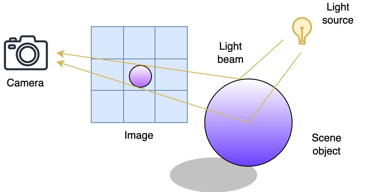
Figure 1:The Rendering Process and Its Key Components. The camera captures the scene by tracing rays through pixels in the image, interacting with objects and light sources to determine the final colors. In short, rendering simulates the physics of light to produce realistic or stylized images.
In code, rendering typically starts with defining a scene containing objects, lights, and a camera. A simple example in Python using a ray tracing approach might involve casting rays from a virtual camera, checking for intersections with scene objects, and computing shading based on light interactions. In this chapter, we will first introduce the simpler method: rasterization and then we will dive deep into ray tracing. By the end of this chapter, readers will have an overview of what is rendering and may create their own renderers for customized OpenUSD workflows.
11.2 Fast Rendering by Rasterization
Rasterization is a rendering technique that converts 3D objects into pixels on a 2D screen by projecting their geometry and filling in the appropriate pixel values. It works by taking the vertices of a 3D model, transforming them through a camera projection, and then breaking down the shapes into fragments that correspond to pixels. A key step in rasterization is determining which pixels belong to a given triangle and how to shade them based on lighting and textures. Unlike ray tracing, which simulates light rays, rasterization approximates lighting calculations, making it computationally efficient.
The main benefits of rasterization are speed and real-time performance, making it the preferred choice for applications like video games, interactive graphics, and real-time simulations.
Let’s first ensure that we have the following two packages numpy and PIL(pillow) to perform numerical computing and operating images. If not so, readers can install them via (pip install numpy pillow) in the command line.
import numpy as np
from PIL import Image
In this section, we are going to write a Python render for a simple mesh in .usd format. Let’s get started by downloading the .usd (https://
from pxr import Gf, Usd, UsdGeom, Sdf

stage = Usd.Stage.CreateNew("render.usd")

# Move xform to -z axis
xform = UsdGeom.Xform.Define(stage, '/World/icosphere')
xform.AddTranslateOp().Set(Gf.Vec3f(0, 0, -5))

prim = xform.GetPrim()

# Import asset
prim.GetReferences().AddReference(assetPath="<your path to icosphere.usd>")
Now, we have an icosphere on the stage. To take a picture of it using script, we have to first find out its geometric properties such as vertices and faces. The following code retrieves essential geometric data from a mesh object. mesh.GetPointsAttr().Get() extracts the list of vertex positions in 3D space, typically as an array of Gf.Vec3f values. mesh.GetFaceVertexCountsAttr().Get() retrieves the number of vertices per face, where each entry represents the number of vertices in a corresponding face (e.g., 3 for triangles, 4 for quads). Finally, mesh.GetFaceVertexIndicesAttr().Get() obtains the indices that define the connectivity of the mesh, mapping vertices to faces by referencing their positions in vertex_points. Together, these attributes define the mesh’s geometry, allowing for further processing, rendering, or transformations. (Readers can review Chapter 4 for more details.)
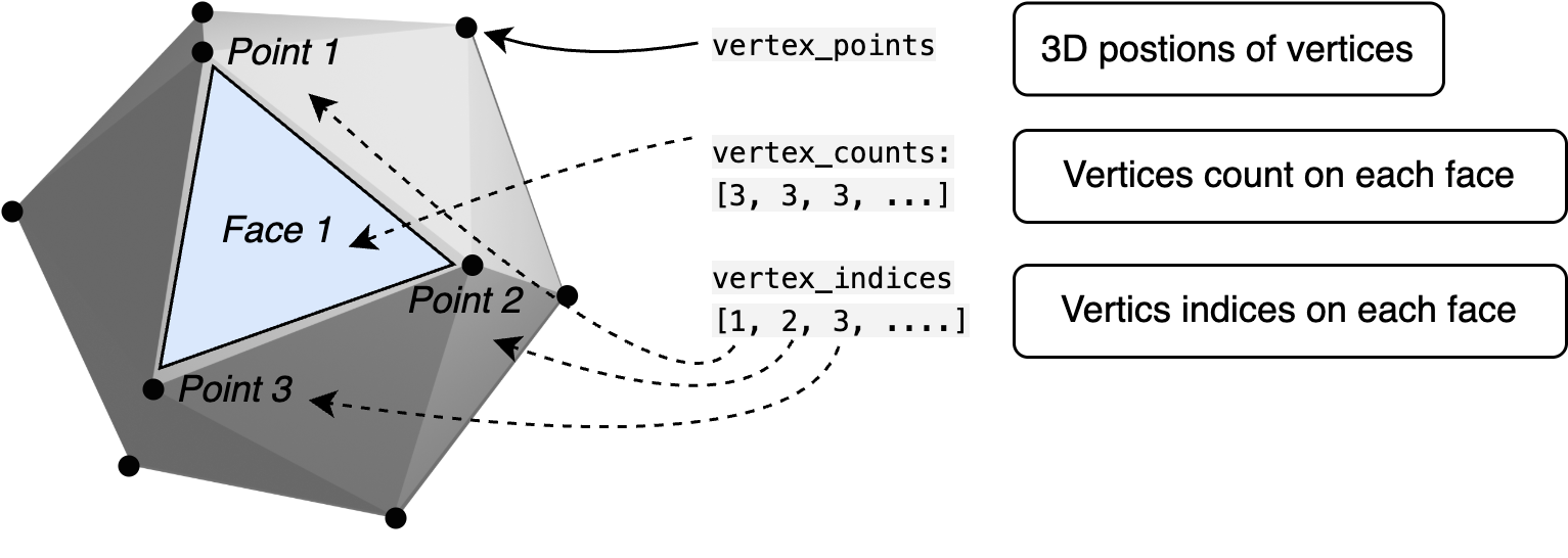
Figure 2:Accessing Mesh Data. Using the OpenUSD API, we can access a mesh’s vertex positions, face vertex counts, and face vertex indices. These attributes define the mesh’s structure, enabling further processing for rendering or geometry manipulation.
mesh = UsdGeom.Mesh.Get(stage, "/World/icosphere/Icosphere/mesh")

# Access mesh vertex data: points, face counts, and indices
vertex_points = mesh.GetPointsAttr().Get()
vertex_counts = mesh.GetFaceVertexCountsAttr().Get()
vertex_indices = mesh.GetFaceVertexIndicesAttr().Get()
However, the above vertex_points contain only the point location in the mesh local space, we have to know it world coordinates:
vertex_points = [v + xform.GetTranslateOp().Get() for v in vertex_points]
eye = Gf.Vec3f(0, 0, 1)
Now, let’s place an eye (or camera) at position (0, 0, 1), looking in the -z direction. From this viewpoint, the camera should see the icosphere positioned at (0, 0, -5). But how do we display this on a 2D screen? Suppose we position a 2D screen on the x-y plane with its origin at (0,0,0). To project a point from 3D space onto this screen, we find the intersection between the line connecting the eye and the point and the plane of the screen. This process simulates how a 3D scene is captured and displayed in a 2D image.
# Convert 3D point to 2D screen coordinates
def point_to_screen(point: Gf.Vec3f) -> Gf.Vec2f:
    d = (point - eye).GetNormalized()
    t = - eye[2] / d[2]
    x = eye[0] + t * d[0]
    y = eye[1] + t * d[1]
    return Gf.Vec2f(x, y)
We define a function point_to_screen to project a 3D point onto a 2D screen using a simple perspective projection. First, it computes the direction vector d from the eye (camera position) to the given point, normalizing it to ensure a consistent scale. Then, it determines the intersection of this direction with the x-y plane (screen) by solving for t using the equation z = 0, derived from the parametric line equation
The computed t value represents the distance along the ray at which it meets the screen. Finally, the function calculates the x and y coordinates of the intersection and returns them as a 2D point in screen space:
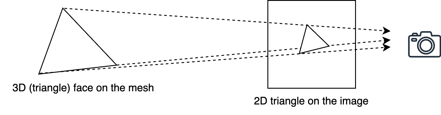
Figure 3:Projecting 3D Vertices to 2D Screen Space. Using a camera’s perspective projection, each 3D point is mapped onto a 2D plane, simulating how a scene is viewed from a specific vantage point. This step is essential in rendering, as it converts spatial geometry into an image representation.
screen_points = [point_to_screen(p) for p in vertex_points]Then we assume a 2D coordinate screen (canvas) where the top_left and bottom_right points define a square region. The top left corner is at (-0.2, 0.2) and the bottom right corner is at (0.2, -0.2), meaning the square spans from -0.2 to 0.2 in both the x and y directions. The resolution is set to 256, suggesting that the space will be discretized into a 256 by 256 grid. The delta value, calculated as (0.2 + 0.2) / resolution, represents the step size between grid points, determining the spacing of samples along each axis.
top_left = Gf.Vec2f(-0.2, 0.2)
resolution = 256
delta = (0.2 + 0.2) / resolution
To get the pixel position on the screen, we define a function:
def pixel(i, j):
    return top_left + Gf.Vec2f(i * delta, - j * delta)
Now, to determine the color of each pixel, we first need to identify which polygons from the 3D scene are projected onto our 2D screen. Since all polygons in our case are triangles, we can find their positions by extracting the corresponding vertices. Each triangle is defined by three indices stored in vertex_indices. By grouping these indices in sets of three, we can retrieve the vertex positions from screen_points, forming a list of triangles that define the scene on our screen.
Here’s the code that accomplishes this:
polygons = [[screen_points[idx] for idx in vertex_indices[3 * i:3 * i + 3]] for i in  range(len(vertex_counts))]
```python

This code loops through all triangles, extracts the three vertex positions for each, and stores them in polygons, which will be used for rendering.

To correctly render the scene, we need to determine the depth of each polygon, which tells us how far it is from the camera. Since multiple polygons can overlap on the 2D screen, depth information helps us decide which ones should be visible and which should be hidden behind others (a process known as depth sorting or z-buffering). The following code calculates the average depth of each triangle:To determine the color of each pixel on the screen, we first need to check whether a pixel lies inside a polygon.
```python
polygon_depth = [np.mean([vertex_points[idx][2] for idx in vertex_indices[3 * i: 3 * i + 3]]) for i in range(len(vertex_counts))]
To simplify the rendering process in our case, we assign each polygon a random color. The following code generates random RGB values (ranging from 0 to 256) for 20 polygons:
polygon_color = [Gf.Vec3f(np.random.rand()*256, np.random.rand()*256, np.random.rand()*256) for i in range(len(vertex_counts))]Note In most rendering systems, the color of a polygon is determined by complex shading techniques, such as lighting calculations, texture mapping, or material properties. These methods take into account factors like light sources, surface normals, and reflections to create realistic images.
Since our rendering process involves filling triangles with color, we need to define a function for deciding which pixels should be colored based on their position relative to the projected polygons.
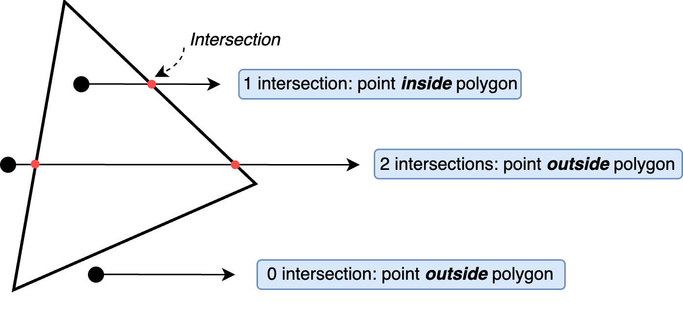
Figure 4:Odd-Even Rule for Point-in-Polygon Test. By drawing a horizontal ray from the point and counting its intersections with the polygon’s edges, the rule states that an odd number of intersections indicates the point is inside, while an even number means it is outside. This technique is fundamental in computational geometry and rasterization.
The following function works by iterating through the edges of a given polygon and checking how many times a horizontal ray, extending from the pixel to the right, crosses the polygon’s edges. If the ray crosses an odd number of times, the pixel is inside the polygon; otherwise, it is outside. This logic is implemented using a loop that examines the y-coordinates of the polygon’s edges and determines whether the horizontal ray from the pixel intersects the edge. If an intersection is found, the inside flag is toggled. By the end of the loop, the function returns True if the pixel is inside the polygon and False otherwise. This method ensures accurate rasterization of polygons on the screen.
def is_pixel_in_polygon(pixel, polygon) -> bool:
    x, y = pixel
    num_vertices = len(polygon)
    inside = False

    # Iterate through each edge of the polygon
    j = num_vertices - 1  # Previous vertex index

    for i in range(num_vertices):
        xi, yi = polygon[i]
        xj, yj = polygon[j]

        # Check if the point crosses an edge
        if ((yi > y) != (yj > y)) and \
                (x < (xj - xi) * (y - yi) / (yj - yi) + xi):
            inside = not inside

        j = i  # Move to next edge
    return inside
For example, we can check if the top left corner of our screen is contained in the first polygon:
print(is_pixel_in_polygon(pixel(0, 0), polygons[0])) # should print `False`Finally, we can create an RGB image to show the render result:
image_data = np.zeros(shape = (resolution, resolution, 3), dtype=np.uint8)=
for i in range(resolution):
    for j in range(resolution):
        pixel_color = Gf.Vec3f(0, 0, 0)
        depth = -1e6

        for k in range(len(polygons)):
            polygon = polygons[k]

            if is_pixel_in_polygon(pixel(i, j), polygon):
                if polygon_depth[k] > depth:
                    depth = polygon_depth[k]
                    pixel_color = polygon_color[k]

        image_data[i][j] = pixel_color
The above code snippet is responsible for determining the color of each pixel in the final image by checking which polygon is visible at that pixel. It works by looping through every pixel in a resolution × resolution grid, initially setting its color to black (0,0,0) and assigning a very low depth value (-1e6) to track the closest polygon. For each pixel, it checks all polygons to see if the pixel is inside one using is_pixel_in_polygon(). If the pixel belongs to multiple overlapping polygons, the code compares their depth values (polygon_depth[k]) and selects the one that is closest to the eye at (0, 0, 1). The pixel’s color is then updated to match the color of the closest polygon. Finally, the chosen color is stored in image_data[i][j], creating the final rendered image.
Note While the odd-even rule is a simple and intuitive method for determining whether a point is inside a polygon, it can be computationally inefficient, especially for complex or highly detailed meshes. The need to trace a ray and count intersections for each point makes it less practical for performance-critical applications. In real-world scenarios, alternative methods such as barycentric coordinates (Barycentric coordinate system) offer more efficient and numerically stable solutions, particularly for triangles, by directly computing the point’s position relative to the polygon’s vertices. Other techniques, like the winding number algorithm, may also be preferred for handling concave polygons or those with holes more robustly.
The following code shows the image:
image = Image.fromarray(image_data, mode="RGB")
image.show()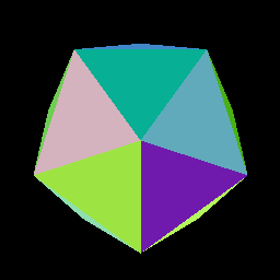
Figure 5:Rendering Results of an Icosphere.
11.3 Rendering via Ray Tracing
Rendering via ray tracing is a technique that simulates the way light interacts with objects to produce highly realistic images. Unlike rasterization, which processes geometry in a top-down manner by projecting triangles onto a screen, ray tracing follows the path of light as it travels through a virtual scene. It traces rays from the camera into the scene, checking for intersections with objects and computing how light interacts with surfaces. This approach enables accurate reflections, refractions, soft shadows, and global illumination, making it widely used in high-end visual effects, photorealistic rendering, and real-time applications with modern GPU acceleration.
A key advantage of ray tracing is its ability to naturally handle complex lighting effects that are difficult to achieve with traditional rasterization. By simulating light transport, ray tracing can produce physically accurate images with realistic shading and material properties. However, the computational cost is significantly higher, requiring optimizations like bounding volume hierarchies (BVH) to accelerate ray-object intersection tests. With recent advancements in hardware, such as dedicated ray tracing cores in GPUs, real-time ray tracing has become more feasible, bridging the gap between offline cinematic rendering and interactive applications like video games.
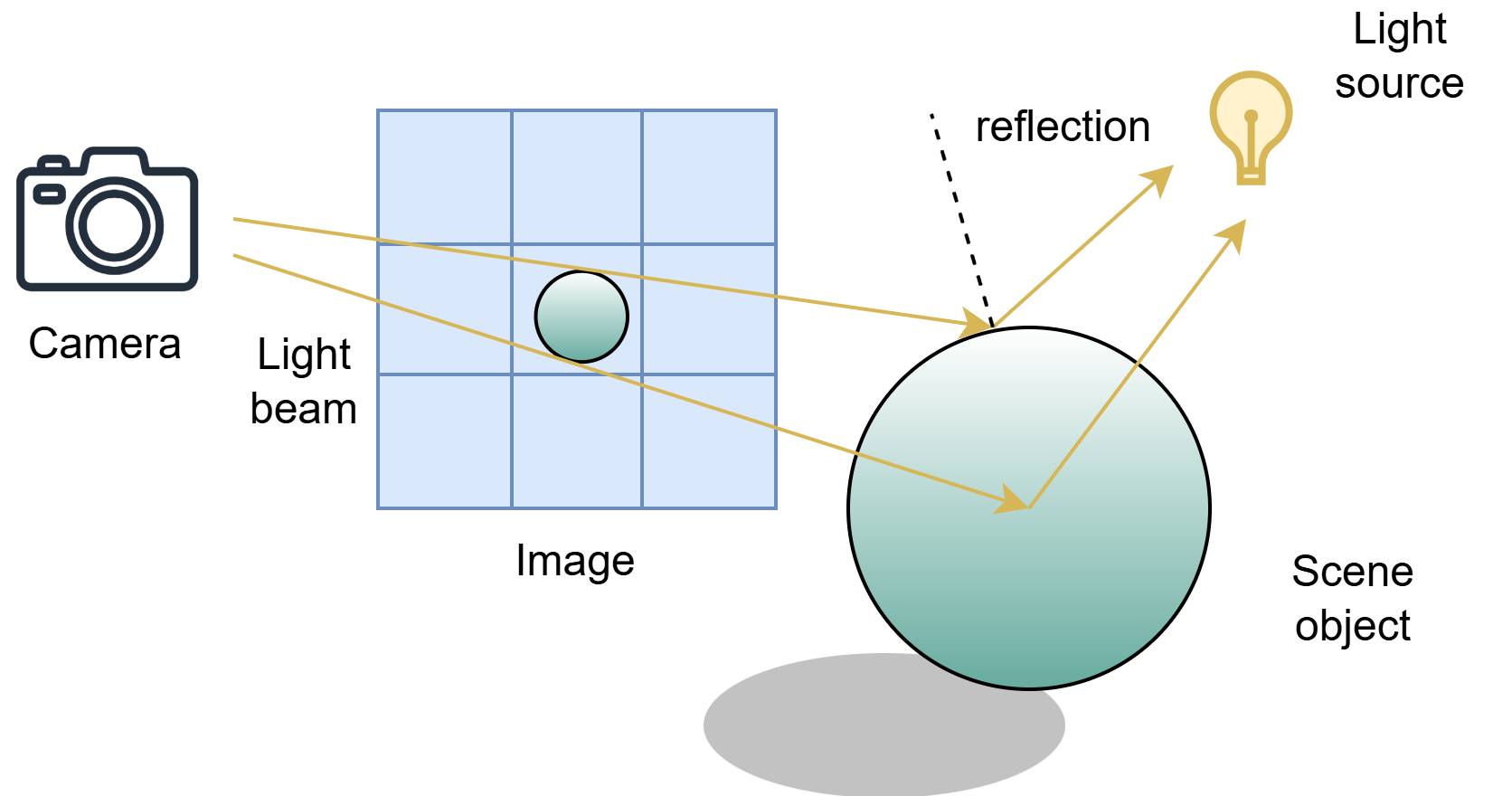
Figure 6:The Ray Tracing: shooting a light from the camera to find a light source. While rasterization projects geometry directly onto the screen, ray tracing simulates the paths of individual rays to achieve more realistic lighting, reflections, and shadows.
In this section, let’s do a simple practice to illustrate the key idea of ray-tracing rendering. Again, we are going to use the icosphere. Here, we can copy and paste some of the code from the previous section:
import numpy as np
from PIL import Image
from pxr import Gf, Usd, UsdGeom, Sdf

stage = Usd.Stage.CreateNew("render.usd")
xform = UsdGeom.Xform.Define(stage, '/World/icosphere')
xform.AddTranslateOp().Set(Gf.Vec3f(0, 0, -5))

prim = xform.GetPrim()
prim.GetReferences().AddReference(assetPath="./icosphere.usd")

mesh = UsdGeom.Mesh.Get(stage, "/World/icosphere/Icosphere/mesh")

vertex_points = mesh.GetPointsAttr().Get()
vertex_counts = mesh.GetFaceVertexCountsAttr().Get()
vertex_indices = mesh.GetFaceVertexIndicesAttr().Get()
vertex_points = [v + Gf.Vec3f(xform.GetTranslateOp().Get()) for v in vertex_points]
In rasterization, the goal is to quickly project 3D geometry onto a 2D screen by calculating pixel coverage, but in ray tracing, the process is different: it requires working directly with 3D triangles to simulate how light rays interact with surfaces. Instead of just finding where geometry appears on the screen, ray tracing casts rays into the scene, checks for intersections with 3D triangles, and calculates reflections, refractions, and lighting based on surface properties. In the following code, triangles are reconstructed from vertex points and indices, preparing the 3D geometry for accurate ray-triangle intersection tests needed for realistic lighting effects.
triangles = [[vertex_points[idx] for idx in vertex_indices[3 * i:3 * i + 3]] \
    for i in range(len(vertex_counts))]
Again, we set up the “screen” we need to capture the image. However, since we want the screen in 3D space to calculate the ray direction:
top_left = Gf.Vec3f(-0.2, 0.2, 0)
resolution = 256
delta = (0.2 + 0.2) / resolution
In the real world, our eyes receive light that reflects off objects around us. In ray tracing, we reverse this process: we imagine rays of light starting from the eye and traveling outward into the scene, searching for surfaces and light sources to create the final image. For example, if compose a light ray shooting from the eye to the top left corner of the screen, the origin of the ray the position is the eye, and the direction (normalized into unit vector) should be
d = (top_left - eye).GetNormalized()Now it’s time to dive into some math. At the heart of ray tracing lies a simple but powerful question: where does the light ray travel? To answer this, we need to solve two key problems: (1) determine whether a ray intersects with any part of the mesh, and (2) if an intersection occurs, calculate the direction of the reflected light.
To calculate whether the ray intersections with a triangle in 3D space, we apply the Möller–Trumbore intersection algorithm.
The Möller–Trumbore algorithm is a simple and efficient method used in ray tracing to determine whether a ray of light hits a triangle, which is a common shape used to build 3D objects. Instead of testing complex equations for every possible intersection, this algorithm directly uses the triangle’s corners and the ray’s path to quickly decide if they meet.
Below is the function, which you can think of as a helper that determines whether a ray—with a given origin and direction—intersects a triangle defined by vertices (v0, v1, v2). If an intersection occurs, the function returns true along with the intersection point; otherwise, it returns false. For those interested in the underlying mathematics, please refer to the Wikipedia page for the Möller–Trumbore intersection algorithm: https://en.wikipedia.org/wiki/Möller–Trumbore_intersection_algorithm.
def ray_triangle_intersect(orig, dir, v0, v1, v2):
    """
    orig: ray origin
    dir: ray direction (normalized)
    v0, v1, v2: vertices of the triangle
    """
    EPSILON = 1e-6

    # Find vectors for two edges sharing v0
    edge1 = v1 - v0
    edge2 = v2 - v0

    # Begin calculating determinant - also used to calculate u parameter
    h = Gf.Cross(dir, edge2)
    a = Gf.Dot(edge1, h)
    if -EPSILON < a < EPSILON:
        return False, None  # This ray is parallel to this triangle.

    f = 1.0 / a
    s = orig - v0
    u = f * Gf.Dot(s, h)

    if u < 0.0 or u > 1.0:
            return False, None

    q = Gf.Cross(s, edge1)
    v = f * Gf.Dot(dir, q)

    if v < 0.0 or u + v > 1.0:
        return False, None
    t = f * Gf.Dot(edge2, q)

    if t > EPSILON:  # ray intersection
        intersection_point = orig + dir * t
        return True, intersection_point
    else:
        return False, None
Program 1:Möller–Trumbore Intersection Algorithm
For example, we can test this function by running the following script:
v0, v1, v2 = triangles[0]
hit, point = ray_triangle_intersect(eye, d, v0, v1, v2)
The output should be (False, None), suggesting the ray shooting from the eye to the top left corner of the screen does not have any intersection with the first triangle.
Next, we need to know whether the ray goes if it meets a triangle. Here we would like to introduce face normals.
In OpenUSD, the face normal of a mesh refers to a vector that is perpendicular to the surface of a polygon, typically a triangle or quad. This normal represents the overall direction the face is pointing and is important for calculating lighting, shading, and reflections. However, in real-world OpenUSD workflows, it’s more common to use vertex normals instead of face normals. Vertex normals are smoother because they are averaged across adjacent faces, allowing for softer lighting transitions and more natural-looking surfaces, especially on curved models.
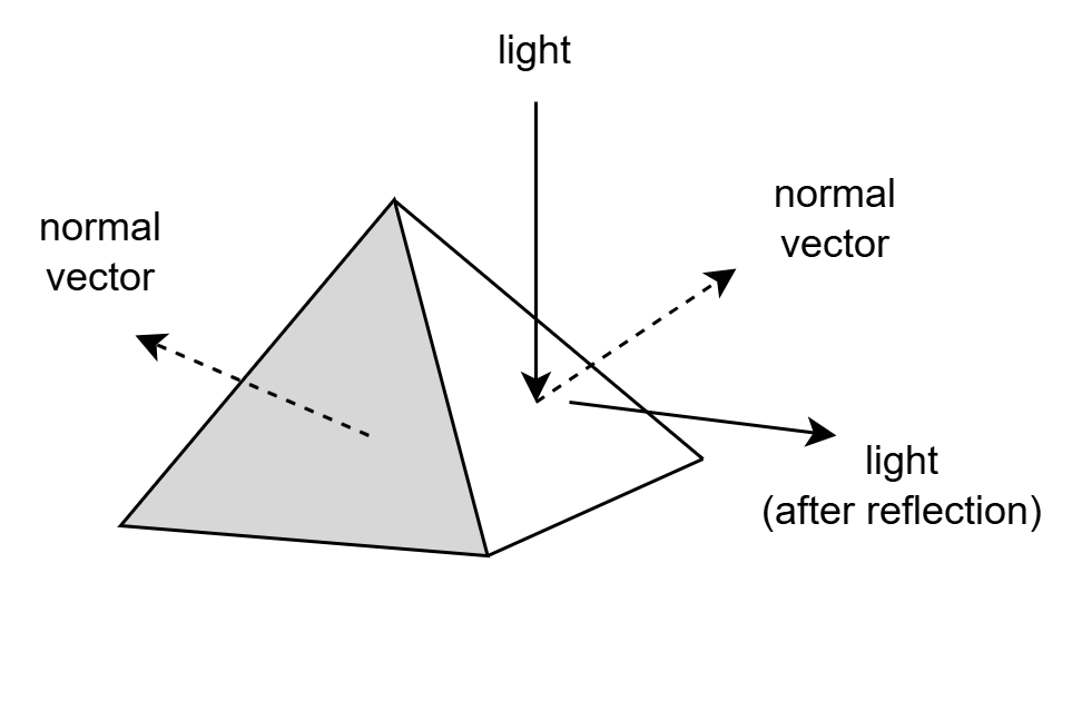
Figure 7:Face Normal and Light Reflection. The face normal is perpendicular to the surface and plays a key role in determining the direction of the reflected light, which is essential for realistic shading and rendering.
For our simple case, the vertex and face normal of the triangles are the same. We can just pick one vertex normal for calculation. For example, the following code gets the normal vector of the first triangle.
vertex_normals = mesh.GetNormalsAttr().Get()
triangle_normal_0 = vertex_normals[0:3][0]
Here we need to apply the reflection law learnt from middle school: when light strikes a smooth, reflective surface, the angle of reflection is equal to the angle of incidence. Or in math:
def reflect(dir, normal):
    """
    Reflects a direction vector 'dir' around the given 'normal'.
    Both should be normalized!
    """
    return dir - 2 * Gf.Dot(dir, normal) * normal
Program 2:Reflection Law
The function returns the reflected direction of the ray given the normal vector of a face.
Finally, suppose we have a direction light. The pixel color is then approximated by this alignment: brighter if the reflection faces the light, or darker otherwise. For example, given a direction light and a reflected light ray, we can decide the pixel color by:
direction_light = Gf.Vec3f(1, 1, 1).GetNormalized()
ray = Gf.Vec3f(0, 0, 1)
color = Gf.Dot(direction_light,ray)
Finally, we can perform a basic form of ray tracing to approximate the color of each pixel in an image based on the direction of incoming light. Similarly, let’s define an image to store the color data:
image_data = np.zeros(shape = (resolution, resolution, 3), dtype=np.uint8)For each pixel, it casts a ray from the camera (the “eye”) through a grid of points in space. It checks if the ray intersects any triangle in the scene using the ray_triangle_intersect function. If an intersection is found and it’s the closest one along the ray, it calculates the triangle’s surface normal, computes the reflection direction, and estimates how much the reflected ray aligns with the light direction.
for i in tqdm(range(resolution)):
    for j in range(resolution):
        d = top_left + Gf.Vec3f(i * delta, - j * delta, 0) - eye
        d = d.GetNormalized()
        depth = -1e6

        for k in range(len(triangles)):
            v0,v1,v2 = triangles[k]
            intersection, point = ray_triangle_intersect(eye, d, v0, v1, v2)
            if intersection:
                if point[2] > depth:
                    depth = point[2]
                    normal = vertex_normals[3 * k]
                    reflected = reflect(d, normal)
                    factor = Gf.Dot(light_dir, reflected)

                    if factor > 0:
                        image_data[i][j] = [255. * factor, 255. * factor, 255. * factor]
                    else:
                        image_data[i][j] = [50, 50, 50]
The image can be shown via the following code:
image = Image.fromarray(image_data, mode="RGB")
image.show()
The result of the ray-tracing rendering is shown in Figure 8 (left). Compared to rasterization, ray tracing typically produces images with greater visual realism, capturing accurate reflections, lighting, and shading effects. However, this improved quality comes at the cost of longer computation times, as ray tracing requires simulating the complex interactions between light and surfaces.
For example, because the object surface is not smooth, in real practices we may add some randomization during light reflections:
def reflect(dir, normal, randomize = True):
    """
    Reflects a direction vector 'dir' around the given 'normal'.
    Both should be normalized!
    """
    reflected_dir =  dir - 2 * Gf.Dot(dir, normal) * normal
    if randomize:
        random_vector = Gf.Vec3f(np.random.randn(), np.random.randn(), np.random.randn())
        reflected_dir = reflected_dir + random_vector

    return reflected_dir.GetNormalized()
Program 3:Reflection with Randomization
Because we add noise to the reflected rays, the rendered image may appear a bit messy, as shown in Figure 8 (middle). However, if we perform many samples per pixel (e.g., 50 samples) and average the results, the noise is significantly reduced, and the image looks much cleaner and more visually appealing.
for i in tqdm(range(resolution)):
    for j in range(resolution):
        d = top_left + Gf.Vec3f(i * delta, - j * delta, 0) - eye
        d = d.GetNormalized()
        depth = -1e6

        for k in range(len(triangles)):
            v0,v1,v2 = triangles[k]
            intersection, point = ray_triangle_intersect(eye, d, v0, v1, v2)

            if intersection:
                if point[2] > depth:
                    depth = point[2]
                    normal = vertex_normals[3 * k]
                    factors = np.zeros(50)
                    for t in range(50):
                        reflected = reflect(d, normal, randomize=True)
                        factors[t] = Gf.Dot(light_dir, reflected)

                    factor = np.mean(factors)
                    if factor > 0:
                        image_data[i][j] = [255. * factor, 255. * factor, 255. * factor]
                    else:
                        image_data[i][j] = [50, 50, 50]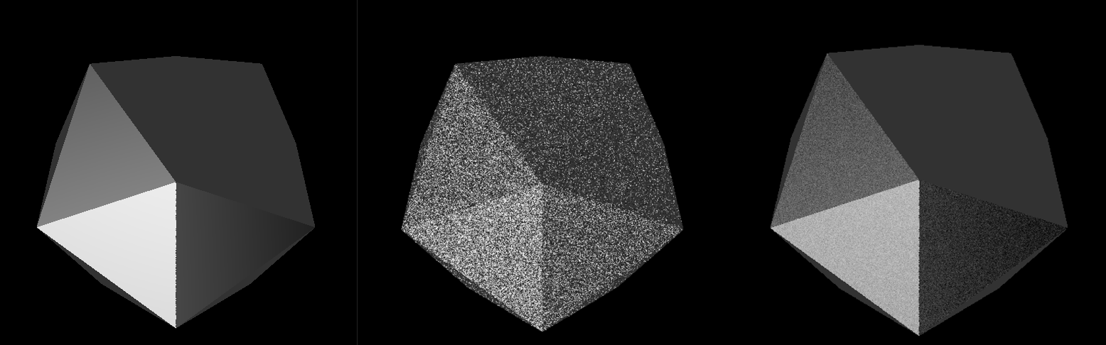
Figure 8:Simplified Ray-Tracing Rendering Results of an Icosphere. The left side does not consider randomization. The middle and right images apply the effect of randomized reflection.
In real-world applications, building a full ray tracer from scratch is rarely necessary. Instead, OpenUSD scenes are typically rendered using professional-grade renderers that already support advanced ray tracing. Popular renderers like HDStorm, Embree, Hydra-based renderers, and third-party options such as RenderMan, Arnold, and Omniverse provide built-in ray tracing capabilities optimized for speed, quality, and scalability. In OpenUSD workflows, Hydra acts as a rendering framework that connects scene data to these high-performance renderers. To take advantage of ray tracing, users simply need to configure their Hydra delegate to use a ray-tracing-capable backend. For example, when working with Omniverse, users can enable real-time RTX ray tracing with just a few settings. Similarly, other renderers often provide options to toggle between rasterization and ray tracing modes depending on the quality and performance needs. In practice, accessing ray tracing through these systems allows artists and developers to achieve photorealistic results without worrying about the complex math behind the scenes.
Summary
- Rendering is the process of converting 3D scene data (like geometry, lights, and materials) into a 2D image that we can view.
- Rasterization is a traditional rendering technique that projects 3D objects onto a 2D screen by quickly determining which pixels correspond to which triangles.
- Ray tracing is a more physically accurate rendering method that simulates the path of light rays as they bounce around a scene. It can produce highly realistic images with reflections, refractions, and global illumination but usually requires more computational time.