This chapter covers
- Preparing our programming environment for using AI
- Automating AI interactions and OpenUSD workflows through Python scripting
- Using natural language prompts to create, edit and interact with USD files
- Creating image textures with generative AI
- Managing and searching 3D assets with AI-powered vector databases

The convergence of AI and 3D graphics is reshaping how we approach content creation and digital pipeline automation. At the heart of this shift is the rapid advancement of large language models (LLMs) and generative AI tools, which have become not only powerful assistants for writing code but also collaborators capable of reasoning about complex file structures, creating or editing .usda files, and generating visual assets. For OpenUSD developers, this new capability can help to streamline production workflows, increase productivity, and reduce the manual overhead traditionally required for building, editing, and managing USD stages.
Despite the potential of AI tools, integrating them into OpenUSD workflows is not straightforward. Developers face a fragmented landscape of APIs, SDKs, and model providers. Each offers unique strengths, but lacks a unified path for interaction with USD scenes. The challenge is not just in accessing these models, but in using them effectively, whether to generate code, interact with complex scenes, or manipulate existing stages using natural language prompts.
We’ll guide you through a structured approach to embedding AI into OpenUSD workflows with Python, addressing the complexities of integration along the way. We’ll begin by setting up the necessary environment to interface with LLMs via the OpenAI SDK and other leading platforms. From there, you’ll learn to:
- Conversationally interact with LLMs (Section 9.2) to generate code or query stage data.
- Write Python scripts for OpenUSD using AI-suggested logic (Section 9.2.2).
- Parse and manipulate USDA files by feeding them into LLMs and interpreting the structured responses (Section 9.2.3).
- Edit stages through natural language inputs, enabling intuitive, high-level control over scene layout and properties (Section 9.2.4).
- Generate image textures with text-to-image models like Flux, or Stable Diffusion, and apply them directly in your stages (Section 9.3).
- Manage and search your 3D assets using vector databases powered by AI-based embeddings (Section 9.4).
By treating LLMs as programmable tools, we move beyond simple text generation and into the realm of intelligent automation. We aim to go beyond basic API usage by providing practical techniques for integrating AI into everyday tasks, helping you automate repetitive work, prototype OpenUSD scenes and scripts quickly, and streamline common workflows through natural language interaction and code generation. The workflows are built on standard Python practices, making them transparent, customizable, and easy to integrate into existing pipelines. You’ll leave with not only working scripts, but a deeper understanding of how AI can serve as a creative and technical ally in OpenUSD development.
Note Appendix D contains supplementary material that will help you navigate the examples in this chapter. We recommend reviewing the sections on creating API keys with OpenAI and/or NVIDIA, as having these set up in advance will ensure a smoother workflow.
10.1 Preparing to Chat with LLM’s
Before integrating an LLM in our 3D workflow, we’ll need to prepare our programming environment and decide which model to connect to via an API:
- Install the OpenAI SDK (Software Development Kit): provides the tools and libraries necessary to interact with AI models programmatically.
- Set up an API key: acts as an authentication token to securely access an LLM.
- Choose an AI model: such as ChatGPT, GPT4o, or Llama3-7B.
Once these steps are completed, we will be fully prepared to harness the power of LLMs to enhance our 3D workflows.
10.1.1 Installing the OpenAI SDK
The OpenAI SDK allows developers to interact seamlessly with OpenAI’s models, such as GPT-4, and a wide range of other AI model resources such as NVIDIA Inference Microservices (NIM). By installing this SDK, we gain access to a range of functionalities that can help automate tasks, generate creative content, and analyze complex data. The SDK simplifies the API interaction process, providing developers with a straightforward way to send requests and receive responses, making it a handy tool for anyone looking to bring AI into their creative pipeline.
Installing the OpenAI SDK is quick and easy. Since it’s a Python package, we can use pip (Python’s package installer) to install it directly into the same virtual environment we set up in Appendix A, where we also installed the use-core package.
Ensure you install the OpenAI SDK and its dependencies before activating Python. In your terminal or command prompt, use the following command:
pip3 install openaiWait for the process to complete, then we can activate the Python interpreter and verify the installation by checking the version of the OpenAI package installed:
pythonimport openai
print(openai.__version__)10.1.2 Configuring API Keys
To securely access AI models from platforms like OpenAI, you’ll need an API key. This unique identifier authenticates your requests, ensuring only authorized users can utilize the models and services. This protects your data and resources from unauthorized access and misuse. Therefore, an API key is often a prerequisite for any application or workflow that interacts with cloud-based AI platforms.
Important Note When generating your API keys, they will only be shown once, so it is important to save them somewhere memorable and secure.
For brevity, we’ll focus on two AI service providers that are typically accepted across industries:
- OpenAI (https://openai.com): A leading AI research organization that provides powerful models like GPT-4 for natural language processing, enabling a wide range of applications from text generation to code assistance.
To get an API key from OpenAI, please visit the API-key-setup page (https://
- NVIDIA Inference Microservices (NIM) (https://
ai .nvidia .com): An advanced AI platform from NVIDIA that combines deep learning, high-performance computing, and generative models to deliver state-of-the-art AI capabilities as foundation models (large, general-purpose models pre-trained on vast datasets, adaptable for various downstream tasks).
To get an API key for foundation models from NVIDIA NIM, please visit the page (https://
10.1.3 Choosing Your Favorite LLM
When selecting a language model for your projects, it’s important to consider the unique features and strengths of each model offered by major providers such as OpenAI, Meta, Google, and Microsoft. Each of these organizations offers advanced LLMs with distinct capabilities and applications, making it important to choose the one that best aligns with your specific needs. Table 1 gives a brief comparison of different models. This is a fast moving industry, so features may change.
Table 1:A brief comparison between different LLMs
| Series | Provider | Features | Model examples |
|---|---|---|---|
| GPT | OpenAI | Most advanced, well-regarded for their versatility in handling a wide range of tasks | gpt-4o, gpt-4o-mini |
| Llama | Meta | More open and accessible | llama 3.1 |
| Gemini | Good integration with Google’s ecosystem | gemini 1.5-pro | |
| Mistral | Microsoft | High flexibility, multi-language ability | Mistral 8x22B |
| Phi | Microsoft | Relatively small, efficient and robust | Phi 3.5 |
10.2 Chatting with LLMs
With LLMs like GPT-4 becoming more powerful and accessible, they offer new opportunities to streamline and elevate the way we work with complex data formats like OpenUSD, allowing you to integrate natural language understanding and generation directly into your tools and applications.
Let’s explore how we can use LLMs with OpenUSD. First, we’ll cover API interactions with OpenAI and NVIDIA NIM. Then, we’ll look at using LLMs to write Python code for OpenUSD, interpret .usda files, and assist with stage editing. By the end of this section, you’ll be able to seamlessly integrate LLMs into your OpenUSD projects for improved productivity.
10.2.1 Conversing with LLMs
To generate a response from an LLM using an API, we need to define a prompt, send it to the model using a request method, and receive a structured response. The prompt is a string containing the input, such as a question, instruction, or description, that we want the model to process. This prompt is sent to the model via an API call, which can be made either directly to a REST endpoint (a specific URL on a web server that is designed to handle requests and responses following the Representational State Transfer architecture, e.g., a URL like https://
Regardless of the method used, the API request typically includes a model parameter to specify which LLM should respond, and a messages parameter to structure the conversation. The messages parameter is usually a list of dictionaries, each representing a part of the dialogue. Each dictionary includes a “role” key (e.g., “user”, “assistant”, or “system”) and a “content” key holding the associated text. For example, {“role”: “user”, “content”: prompt} defines the user’s input before the model processes it.
These roles are crucial because they help the model distinguish between the user’s input, its own responses, and system instructions allowing the model to maintain context over multiple interactions. Once the request is sent, the model processes the input and returns a structured response, which can then be extracted and used in an application.
Important Note Make sure you have some credits available in your OpenAI or NVIDIA NIM account, as the following calls will not work without them. You may need to provide payment details.
Chatting with GPT from OpenAI
To chat with GPT-4o-mini let’s import the OpenAI package, then we can use the API key that we configured earlier to define the client which will allow us to send authenticated requests to the model endpoint:
from openai import OpenAI
client = OpenAI(api_key = <"your_openai_api_key_here">)
Now we’re ready to chat with GPT-4o-mini by providing a prompt and requesting a response via the API using the method call client.chat.completions.create(). The create() method sends a request to the model with the required model and messages parameters and returns the model’s response:
# Defines the user’s input question as a string
prompt = "What is OpenUSD?"

# Calls the API to generate a response from the model
completion = client.chat.completions.create(
    # Specifies the model to use (GPT-4o-mini)
    model="gpt-4o-mini",
    # Defines the conversation context
    messages=[
        # The user’s prompt is sent as a message with role "user"
        {"role": "user", "content": prompt}
    ]
)
This setup allows the model to understand the input provided by the user and generate a relevant response, which is returned as a completion object. To get the response message:
print(completion.choices[0].message.content) This ensures the response is printed to the screen. It will begin something like this:
AI Response Begin [OpenAI ChatGPT gpt-4o-mini]

OpenUSD, or Open Universal Scene Description, is an open-source framework developed by Pixar…etc.

AI Response End
Chatting with LLMs from NVIDIA NIM
Similarly, to chat with the LLMs from NVIDIA NIM, we can still use the openai Python package. However, instead of relying on the default OpenAI endpoint, we’ll specify a custom REST endpoint using the base_url parameter. This tells the client to direct requests to NVIDIA’s deployment of the API at “https://
from openai import OpenAI

# Initializes the OpenAI client object to interact with the API.
client = OpenAI(
    # Sets the base URL for API requests, specifying the endpoint for NVIDIA’s API.
    base_url = "https://integrate.api.nvidia.com/v1",
    # Provides the API key required for authentication with the NVIDIA API.
    api_key = "your_nvidia_api_key_here"  # Replace with your actual API key
)
Now we can provide the prompt and the client.chat.completions.create() method call, using the same structure as we did for the OpenAI call. This time we’ll specify the meta/llama-3.1-405b-instruct model:
# Defines the user’s input question as a string
prompt = "What are the main features of OpenUSD?"

# Calls the API to generate a response from the model
completion = client.chat.completions.create(
    # Specifies the model to use (meta/llama-3.1-405b-instruct)
    model="meta/llama-3.1-405b-instruct",
    # Defines the conversation context
    messages=[
        # The user’s prompt is sent as a message with role "user"
        {"role": "user", "content": prompt}
    ]
)

# Extracts and prints the AI-generated response
print(completion.choices[0].message.content)
This will print the response to the screen as something like:
AI Response Begin [Meta Llama llama-3.1-405b-instruct]
OpenUSD is an open-source software framework for collaborative 3D content creation, originally developed by Pixar…etc.
AI Response End [blank line]
For the rest of the chapter we’ll be using the first method above, however, if you prefer to try working with the models from NVIDIA NIM, you can adapt the methods below to use the second method where we included NVIDIA’s base_url parameter.
10.2.2 Writing Code for OpenUSD
Let’s explore ways to generate code snippets that can be directly used in OpenUSD workflows. For instance, we can prompt an LLM to create a basic scene setup, define geometries, lighting, and more.
To make sure the LLM provides useful code, you can give it instructions at the start using a system message. This sets the context or rules for the LLM’s behavior at the beginning of a conversation. Think of it like giving the LLM a job description so it knows how to generate a more relevant and targeted response, for example: system_message = “You are a helper for coding using Python for OpenUSD.”
We can embed the message into the system role parameter while calling the client.chat.completions.create() method. For example, if we want to use gpt-4o-mini to generate a stage containing some basic geometries, you can try the following code which repeats the approach we used before but adds a system message:
from openai import OpenAI

# Create the OpenAI client with your API key
client = OpenAI(api_key="your_openai_api_key_here")  # Replace with your actual API key

# Defines the system message that instructs the model to focus on assisting with Python coding for OpenUSD.
system_message = "You are a helper for coding using Python for OpenUSD."

prompt = "Create an OpenUSD stage containing some basic geometries."

completion = client.chat.completions.create(
    model="gpt-4o-mini",
    messages=[
        # Adds the system message to set the model's behavior.
        {"role": "system", "content": system_message},
        {"role": "user", "content": prompt}
    ]
)

# Print the AI-generated response
print(completion.choices[0].message.content)
The code above will elicit a response like:
AI Response Begin [OpenAI ChatGPT gpt-4o-mini]:
Certainly! Below is a script that will create a stage containing some basic geometries:

from pxr import Usd, UsdGeom, Gf, Sdf
stage = Usd.Stage.CreateNew("basic_geometries.usd")...

…You can run this script by pasting it into a command terminal…etc.

AI Response End [blank line]
As you can see, the response may contain a lot of additional information but we only need the code snippet. Luckily Python (and other languages) has a solution for this called ‘regular expressions’.
Regular expressions (often abbreviated as regex) are a powerful tool used for searching, matching, and manipulating text based on patterns. They allow you to define complex search patterns, making it easier to work with strings that follow certain formats. In Python, the ‘re’ module is used to work with regular expressions.
To extract just the Python code from the answer, we can use a regular expression that targets the content within the code block. In the following snippet the re.search function looks for a pattern that matches a code block enclosed within triple backticks (```), optionally preceded by “python” to specify the language. The pattern r’(?:python)?\n([\s\S]*?)’ searches for any text following “python” (if present) and captures everything until the closing “```”. If a match is found (code_match), the extracted code is assigned to the variable code using code_match.group(1). If no match is found, it defaults to using the original content variable. This approach ensures that only the relevant code snippet is extracted while ignoring additional text.
Let’s apply it to our example:
# Imports the 're' module for working with regular expressions in Python.
import re

# Searches for code enclosed in triple backticks (optionally labeled with 'python') in the 'response' string using a regular expression.
code_match = re.search(r'```(?:python)?\n([\s\S]*?)```', response)

# If a match is found, extracts the code between the backticks; otherwise, uses the original 'content'.
code = code_match.group(1) if code_match else content

# Prints the extracted code or the original content if no code is found.
print(code)
Figure 1 displays the output after extracting the code snippet. You can simply copy and paste this code into your command line to set up the stage.
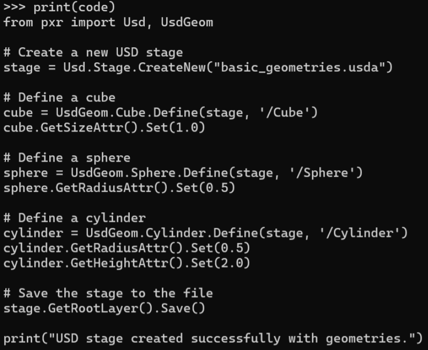
Figure 1:Printed code results from calling OpenAI’s API. By executing the code, you can get a basic_geometries.usda file saved under the working directory.
Incorporating LLMs into our workflow can be extremely useful, especially when we might forget function names or usage details related to OpenUSD. The model’s ability to provide accurate code and documentation helps streamline workflows and ensures you have the information you need at your fingertips.
10.2.3 Talking with LLMs about USDA Files
Thanks to the human-readable format of .usda files, LLMs can parse and understand them, facilitating tasks like generating and interpreting commands, suggesting modifications, and providing content-based insights. Let’s try it out using an example .usda file, shown in Figure 2, named ‘Desktop.usda’, and located within the ‘Ch010’ directory on our GitHub, accessible here: https://
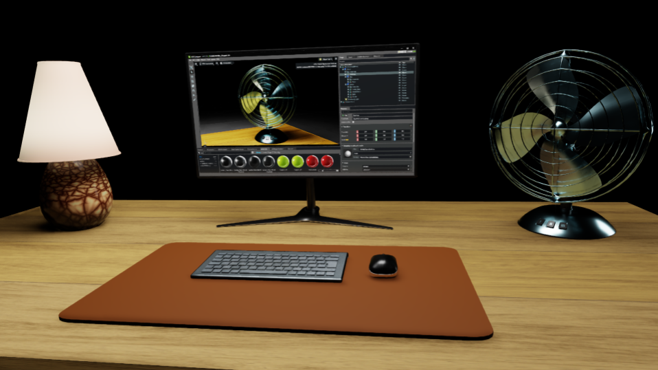
Figure 2:A rendering of the Desktop.usda file. The stage is composed of a desk, a fan, a monitor, and more.
To enable the LLM to read the .usda, we’ll want to structure the message using the system, and user roles. Before that, let’s define the path ‘usd_file_path’ for our file and then use open() to read its content into the ‘usda_content’ variable. The ‘r’ in open(usd_file_path, ‘r’) is a mode specifier that tells Python to open the file for reading only, preventing modification:
from openai import OpenAI

# Create the OpenAI client with your API key
client = OpenAI(api_key="your_openai_api_key_here")  # Replace with your actual API key

# Define the file path to the .usda file
usd_file_path = "./Desktop.usda"  # Replace with your actual path

# Open the file in read ('r') mode
with open(usd_file_path, 'r') as file:
    # Read the entire content of the .usda file into a string
    usda_content = file.read()
Next, let’s structure this interaction by creating a messages list. The first entry in this list will be a dictionary defining the “system” role, which sets the LLM’s behavior as an ‘expert on USDA and OpenUSD stages’. The second element, “role”: “user”, provides the LLM with the actual content of your .usda file by referencing the ‘usda_content’ variable within an f-string. The f before the string is what indicates an f-string, and it allows the code to embed the value of the ‘usda_content’ variable (containing the text of the .usda file) directly into the string that forms the content of the “user” message. This makes it easy to include the file’s entire text within the message sent to the LLM. This structured approach allows us to provide the full scene description to the LLM for further interaction:
# Define a list of message dictionaries to structure the conversation with the LLM
messages = [
    # System message setting the LLM’s behavior and expertise
    {"role": "system", "content": "You are an expert on USDA files and OpenUSD stages."},

    # Inserts the content of the USDA file into the prompt using an f-string
    {"role": "user", "content": f"The following is the content of a USDA file:\n\n{usda_content}"}
]
Now we’re ready to query GPT about the contents of the .usda file. Let’s begin by prompting it to describe the stage. Note that the messages.append() line adds a new dictionary (representing another user message) to the existing messages list.:
prompt = "Briefly describe this stage."

# Append the user message to the existing messages list for the LLM
messages.append({"role": "user", "content": prompt})

# Call the chat completion API to get a description of the .usda stage
completion = client.chat.completions.create(
    model="gpt-4o-mini",
    messages=messages
)

response = completion.choices[0].message.content

print(response)
This will print something like:
AI Response Begin [OpenAI ChatGPT gpt-4o-mini]

This USD stage represents a 3D scene defined as "World," which contains various objects and elements typically found on a desktop setup…

Several objects are defined, each with their transforms and properties: **Desk**: Contains sub-components such as "Fan," "Lamp," "Monitor," "Mat," "Mouse," and "Keyboard…etc.

AI Response End [blank line]
We can also ask GPT other more specific questions. Perhaps we want to learn the transformation data of an object on the stage. Let’s try it with the Fan:
prompt = "Tell me the transformation of the Fan"

# Append the user message to the existing messages list for the LLM
messages.append({"role": "user", "content": prompt})

# Call the chat completion API to get the transformation information
completion = client.chat.completions.create(
    model="gpt-4o-mini",
    messages=messages
)

response = completion.choices[0].message.content

print(response)
This will elicit a response such as:
AI Response Begin [OpenAI ChatGPT gpt-4o-mini]

The "Fan" is defined as a transform node within the "Desk" Xform in the given USD stage. Its transformation parameters are as follows: - **Rotation**: The fan is rotated around the Y-axis by -40 degrees:  ```plaintext  xformOp:rotateXYZ = (0, -40, 0)  ```…

…In summary, the "Fan" is positioned at (0.7, 0.03, -0.2), rotated -40 degrees around the Y-axis, and uniformly scaled with no change to its original size…etc.

AI Response End [blank line]
Again, we might want to extract specific types of information from this full text response. Let’s use the same regex approach we used earlier to extract pure code from a wordy LLM response. This time, the LLM’s response has conveniently enclosed all the Fan’s transform data within triple backticks, so we can adjust the regex to match any text inside triple backticks:
import re    #A

#B Search for all code blocks enclosed in triple backticks (optionally labeled 'plaintext')
transform_matches = re.findall(r'```(?:plaintext)?\n([\s\S]*?)```', response)

#C If any matches are found, join them with double newlines; otherwise, provide a fallback message
transform_data = "\n\n".join(transform_matches) if transform_matches else "No transform data found."

#D Print the extracted transform data
print(transform_data)
Running this script should give us something like the text shown in Figure 3
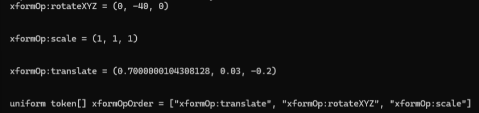
Figure 3:The result of using regex to extract the Fan’s transform data from the full text of the LLM’s initial response.
Interacting with USDA files using LLMs offers significant potential for automating, understanding, and improving scene management in OpenUSD workflows. Processing these complex structures with natural language allows users to streamline tasks and reduce manual effort, opening up new creative avenues. For instance, a useful application might be editing a stage using natural language. Let’s explore how this can be done.
10.2.4 Editing the Stage with LLMs
LLMs offer an intuitive way to edit USD stages by enabling natural language modification of scene elements, properties, and layouts, reducing the need for intricate coding. This conversational approach simplifies workflows, allowing for real-time changes and enhancing creative scene management.
Let’s try modifying our Desktop.usda with a more complex prompt. We’ve added specific requests at the end of the prompt to guide the LLM, helping it stay focused on using the correct syntax for editing the .usda file:
prompt = “Please rotate the Fan and Keyboard by 30 degrees along the up-axis, move the monitor to the right by 0.15 units, and change the Overhead Light intensity into 3000. Please print the updated .usda file. Only use valid USD syntax when updating the .usda file. Make sure not to use expressions like ‘40 + 30’ in transformation values. Provide explicit values instead of combining them.”
messages = [
        {"role": "system", "content": "You are an expert on USDA files and USD stages."},
        {"role": "user", "content": f"The following is the content of a USDA file:\n\n{usda_content}"}

]

messages.append({"role": "user", "content": prompt})

completion = client.chat.completions.create(
        model="gpt-4o-mini",
        messages=messages
)

response = completion.choices[0].message.content
print(response)
Note The more complex our prompt, or the task we are requesting, the longer we may have to wait for a response when we call the client.chat.completions.create method. So be prepared for a pause during the execution of this script.
To extract the usda part of the response, we can use regex again:
# Search for content inside triple backticks (optionally labeled 'usda') in the response
usda_match = re.search(r'```(?:usda)?\n([\s\S]*?)```', response)

# Extract the matched content inside the backticks or set 'content' if no match is found
usda_text = usda_match.group(1) if usda_match else content
Finally, we can save the updated stage into another .usda file. This code opens a file called ‘updated_desktop.usda’ in write mode (“w”) and writes the usda_text content to it. If the file does not exist, it will be created. Once the text is written, the file is automatically closed:
# Open the file "updated_desktop.usda" in write mode ('w'), creating it if it doesn't exist
with open("./updated_desktop.usda", "w") as file:
    # Write the content of 'usda_text' to the file
    file.write(usda_text)
We can now open the stage in our viewer and see the changes made by the LLM. Figure 4 shows the updated stage.
Note At present, there is always the potential for any LLM to misunderstand a request in a prompt, or make syntax errors when writing .usda files. When this happens we may find unexpected results on a stage, or even .usda files that will not open due to errors. If this happens, we can try refining or clarifying our prompts with clearer instructions, or even examining the .usda text output and seeing if we can identify what is wrong before re-prompting with guidance to avoid repeating the error.
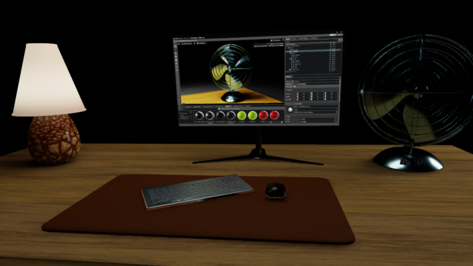
Figure 4:The updated Desktop.usda file. The fan and keyboard are rotated by 30 degrees around the up-axis. The monitor is moved to the right by 0.15 units. The intensity of the overhead light is decreased to 3000.
LLMs provide a fast and intuitive way to edit OpenUSD stages, simplifying tasks like adjusting object properties and transforming layouts through natural language. While they are powerful, errors can occur, and refining prompts may be needed to achieve the desired results. However, with the rapid evolution of this technology, improvements are expected, expanding creative possibilities in digital content creation.
Next, let’s move away from the language models for a moment, and explore how AI image generation might be incorporated into our OpenUSD workflows.
10.3 Generating Image Textures
Currently, AI image generation has limited use in 3D workflows due to the complex and precise way images tend to be applied in 3D. For instance, recall Figure 13 and Figure 14 from Chapter 4 which showed the UV map and image textures of the ring model. Because the UV map dictates the exact placement of texture details on the model, prompting an AI to generate an image that perfectly fits a specific UV map is challenging. This difficulty is amplified when multiple image textures, i.e., Diffuse, Roughness, Metallic, etc. are intended to overlay each other perfectly. In addition, high resolution textures are needed for prominent objects to look good, but most AI image generators only produce 1K or 2K images, and upscaling can cause unwanted variations, hindering perfect texture overlays.
The simpler ‘2D’ or flat elements in a scene are most likely to be suitable for AI generated textures. For example, a monitor screen (like the one in our desktop.usda), a poster, painting, wall, or floor, will generally have straightforward UV maps suitable for applying generated textures. However, this does depend on how the model has been constructed and it will not work for all models. Additionally, generated images can function as backdrops in 3D scenes. For static shots or those with limited camera movement, this is akin to a theatre’s stage backdrop. For shots with more camera rotation a 360° environment texture could work, but achieving seamless edges with AI generation is often difficult, and the low resolution will likely result in a pixelated background. However, depth of field can be used to slightly blur the background and mitigate the visual impact of a low resolution.
Despite these current limitations, AI image generation does have some uses for specific aspects of 3D creation. Given the rapid advancements in this field, we anticipate a much wider integration of generated images into 3D workflows soon. To prepare for this potential, we will include demonstrations of scripting for these types of outputs.
Once we’ve generated an image, we will want to save it by extracting its URL from the AI’s response and downloading it from there. We can do this manually by pasting the URL into a browser, but we will also introduce a method for doing it programmatically by installing Python’s requests package which allows scripts to easily communicate with web servers. The requests package must be installed before we have started the Python interpreter, so let’s do that now. Ensuring that we are working in our desired virtual environment, type the following into a command terminal:
pip3 install requestsAlso, later in this section we will require other Python packages called pillow, numpy, and opencv-python, so let’s install these too:
pip3 install pillow numpy opencv-python Note You will probably get some dependency conflict errors during the install of any of these packages, but as long as you get the ‘Successfully installed…’ message then you will be able to access the package. We’ll demonstrate how to use them after we have generated an image.
Next, don’t forget to start the Python interpreter with the python command, and set your working directory to ‘Ch09’.
10.3.1 Creating and Applying a Diffuse Texture
Let’s begin by generating an image to replace the diffuse texture of the monitor screen in our desktop.usda. OpenAI’s image generation model DALL·E 3 will be suitable for this, but we encourage you to experiment with other image generation models from NVIDIA NIM, such as stable-diffusion-xl, as outputs and capabilities vary considerably. First let’s import OpenAI, provide our API key, then define our prompt:
# Replace with your OpenAI API key
from openai import OpenAI

client = OpenAI(api_key="<your_openai_api_key_here>")
prompt = "A minimalistic nature-inspired wallpaper with soft gradients of blue and green, adding a calm ambiance to a modern desk environment."
Next, let’s generate an image from the prompt using the line response = client.images.generate() which initiates the process through the client object. It calls the generate method on the images interface of the client, storing the result in the response variable. We can then provide arguments to specify which model we want to use, the image size, quality, and output number (n). Note that DALL·E 3 will only accept requests for these sizes ‘256x256’, ‘512x512’, ‘1024x1024’, ‘1024x1792’, and ‘1792x1024’. As we are creating an image for a 16:9 monitor, we can opt for 1792x1024. We also have two options for quality, ‘standard’ or ‘hd’. For speed and efficiency in this demonstration we’ll opt for ‘standard’:
# Calls the OpenAI API to generate an image and stores the response
response = client.images.generate(
    model="dall-e-3",
    prompt=prompt,
    size="1792x1024",  # Ratio appropriate for a monitor screen
    quality="standard",  # Opt for 'standard' quality
    n=1,  # Set the number of images to generate
)
Now let’s access the image by extracting its URL. First we’ll import Python’s requests package, then we’ll take the resulting URL of the image via response.data[0].url, and download the actual image data with the requests.get().content method. Next let’s save it as a PNG file named “new_screen_DIFFUSE.png” within the “textures” folder located inside the “Assets” directory of our current working directory. The use of ‘wb’ when opening the file signifies binary write mode, which allows for writing non-text data like images. Finally, the file.write() method will write the image data to the new PNG file:
import requests

# Extracts the URL of the first generated image from the API response
image_url = response.data[0].url

# Downloads the image content from the retrieved URL
image_data = requests.get(image_url).content

# Opens a file named 'new_screen_DIFFUSE.png' in binary write mode
with open('./Assets/textures/new_screen_DIFFUSE.png', 'wb') as file:
    # Writes the downloaded image data to the file
    file.write(image_data)
To apply our new image texture to the monitor in Desktop.usda, we have a choice regarding the scope of the change. Remembering the way referencing works in OpenUSD, it allows us to modify either the original Monitor.usd asset (affecting all references) or just the instance within Desktop.usda (a non-destructive approach). Opting for the latter to preserve the original asset, let’s open the Desktop.usda.
from pxr import Usd

# Open the Desktop.usda using your file path or a relative path
stage = Usd.Stage.Open("<your path to desktop.usda ex: './Desktop.usda'>")
If we were applying this texture to a new model, we would have to follow the process outlined in Chapter 3, Section 3.5. However, here we are simply replacing an existing texture so we can look up the texture’s attribute path in the Desktop.usda, and reset it using the stage.GetAttributeAtPath().Set() method as follows:
# Defines the USD attribute path to modify
attr_path = "/World/Desk/Monitor/materials/Screen/preview_Image_Texture.inputs:file"

# Gets the attribute at the specified path and sets its value to the new image asset path
stage.GetAttributeAtPath(attr_path).Set("./Assets/textures/new_screen_DIFFUSE.png")

stage.Save()
If we now use our viewer to look at the Desktop.usda, we will now see the monitor screen has changed to our new image texture. Interestingly, if we then open the Monitor.usd from the ‘Assets’ folder of ‘Ch09’ we will see the monitor with its original screen preserved, illustration OpenUSD’s ability to allow non-destructive editing. See Figure 5 for a comparison.

Figure 5:The left image displays the original monitor screen which remains unchanged in the Monitor.usd file, while the right image shows the Monitor.usd file as it will appear on the Desktop.usda stage with the AI-generated image texture applied.
The approach outlined above is suitable for models where we know the image texture is being applied to a relatively simple shape, and the UV map has faces that are appropriately arranged. It may even be useful to create background, with the provisos layed out in the introduction to this section.
We can take it step further by generating multiple texture maps that can be used to create a material. If you need to revise the relationship between textures and materials, refer back to Chapter 4.
10.3.2 Generating Multiple Textures for Materials
Given the current limitations of AI image generation, any generated textures are only likely to be useful for materials applied to simple objects with little prominence in a scene, such as walls, or floors. Assets like these commonly require tileable, also known as seamless, textures. These images are specifically created to repeat across a surface, resulting in a continuous pattern free of visible seams or breaks. However, generating tileable textures requires some specialized AI methods and tools, and the results can be unpredictable. Even well-crafted prompts don’t yield the desired results that often. Therefore, be prepared to experiment and iterate to find prompts, settings and methods that suit your specific model and image requirements.
The following workflow is for generating basic textures quickly. The output may be adequate for background use or rapid prototyping; however, it’s not intended for high-quality, production-ready assets. Our aim is to demonstrate foundational techniques that will remain applicable even as AI becomes more advanced in creating textures. Locally run AI tools provide the greatest control for generation, but the set up for this is complex and outside this book’s scope, so we will utilize cloud-based alternatives.
For seamless, tileable textures, we’ve had reasonably consistent results using a Flux model hosted by HuggingFace (https://
HuggingFace gives us access to multiple AI models and tools, and we’re going to use one that is specialized in making seamless textures. You can view the model here: https://
LoRAs (Low-Rank Adaptation models) work by influencing a model’s output towards a particular style or content. Often, a trigger phrase is needed to activate a LoRA’s effect, and for this one, it’s “smlstxtr”. This LoRA specifically fine-tunes the FLUX model to generate seamless and tileable textures. Therefore, for best results, it’s recommended to structure your prompt with “smlstxtr, <>, seamless texture”.
Besides the actual description of the material we’re prompting for, there are several important details to include in any prompt for a tileable material:
- Use the words “seamless” and “tileable” and “texture” explicitly
- Specify “even lighting” to “avoid baked-in shadows”
- Define the color variation (e.g., “natural color shifts without abrupt changes”)
- Request a “flat” or “top-down view” to avoid perspective or images of objects
- Sometimes it will help to state the size of the object, so that scale is appropriate.
Putting all of that together we might structure a prompt something like this:
AI Prompt Begin [blank line]

Generate a seamless, tileable [material type] texture. Ensure it has realistic, even lighting, natural color variation, and no baked-in shadows. The texture should be a flat, top-down view with [specific details like color range, surface imperfections, etc.]. [State the size of the area the texture covers if necessary].

AI Prompt End [blank line]
Let’s try it out by creating a set of image textures that we can apply to the existing material in our example .usda file named ‘Floor.usda’. This is located in the ‘Ch09’ directory on our GitHub. This simple plane is configured to arrange any applied texture in a 2x2 grid, effectively repeating it four times across its surface to provide a clear visualization of the texture’s tileability (See Figure 6). To produce multiple texture images that perfectly overlay each other we will first generate the Diffuse texture. Once we’re happy that the image tiles well we can use additional Python tools to convert that texture into a Normal, and a Roughness map before adding all three to the floor model to create our finished material.

Figure 6:The seamless pattern on the Floor.usd. Left is the individual image texture, Right is the texture repeated four times in a 2x2 grid, showing how it repeats perfectly.
Let’s begin generating the initial diffuse texture by constructing an HTTP POST request to the model endpoint (a method used to send data to a server, typically to submit forms or interact with APIs). We’ll then provide our authorization token, and a payload containing our prompt for a seamless marble stone texture that includes the trigger phrase for the LoRA, and values for the parameters. The request is sent to the model using Python’s requests library, and the resulting image is downloaded and saved locally.
Important Note Models are not always available via HuggingFace for a variety of reasons. We’re going to try accessing a model specialized in seamless textures, however, just in case it is not available, we have included some conditional error handling at the end of this snippet. If you get an error, try rerunning the code, but replacing the API_URL with: API_URL = “https://
import requests    # Imports the 'requests' library to handle HTTP requests.

# Sets the Hugging Face API endpoint for the Flux texture generation model.
API_URL = "https://api-inference.huggingface.co/pipeline/text-to-image/gokaygokay/Flux-Seamless-Texture-LoRA"

# Defines the HTTP headers, including the required Hugging Face API token.
headers = {
    "Authorization": "Bearer <YOUR_HUGGINGFACE_API_TOKEN>"    # Replace with your actual token.
}

# Constructs the payload with the text prompt and generation parameters.
payload = {
    # The generation prompt containing the trigger phrase for the LoRA, 'smlstxtr'
    "inputs": "smlstxtr, seamless, tileable, photorealisitic marble stone floor texture with realistic, even lighting, natural color variation, and no baked-in shadows. The texture should be a flat, top-down view of a 10x10 meter floor, seamless texture",

    "parameters": {
        "guidance_scale": 7.5,    # Controls prompt adherence; higher values stick more closely to the prompt.
        "num_inference_steps": 30,    # The number of diffusion steps (quality vs speed tradeoff).
    }
}

# Send a POST request to the Hugging Face API with the payload.
response = requests.post(API_URL, headers=headers, json=payload)

if response.status_code == 200 and response.headers["content-type"].startswith("image/"):
    # If successful, saves the binary image content to a PNG file.
    with open("./Assets/textures/seamless_texture_SD3-5.png", "wb") as f:
        f.write(response.content)    # Writes the image data.
    print("Image saved.")

elif response.status_code == 503:
    print("Model is currently unavailable (503). This may be due to inactivity or resource limits.")

else:
    # If the request fails, print the error code and message.
    print(f"Unexpected response: {response.status_code}, content type: {response.headers.get('content-type')}")
We can check if our new texture is seamless by using a little Python script that will stitch four copies of the texture together, so we can look at the seams. This is where the Pillow package that we installed earlier comes in handy. The following snippet will load the texture, duplicate it into a 2x2 layout, save, and display the result for evaluation:
from PIL import Image    # Imports the Python Imaging Library (Pillow) module for image processing

# Loads the texture image from disk
img = Image.open("./Assets/textures/marble_texture_DIFFUSE.png")

# Gets the original image's width and height
w, h = img.size

# Creates a blank 2x2 grid, doubling the width and height of the original to hold four copies of the image
grid = Image.new('RGB', (w * 2, h * 2))

# Paste the texture 4 times to make a 2x2 grid (top left, top right, bottom left, bottom right)
grid.paste(img, (0, 0))
grid.paste(img, (w, 0))
grid.paste(img, (0, h))
grid.paste(img, (w, h))

# Save the 2x2 grid as a new image
grid.save("marble_texture_2x2_grid.png")

# Opens the image in your default viewer so you can visually inspect for tiling seams
grid.show()
Examine the texture closely at the intersection of the four tiles. If you notice obvious tiling errors such as abrupt and unintended detail changes, try regenerating the image by re-running the code from the line that begins “payload = {...”. Use a slightly different prompt, or alter the guidance scale value, otherwise you will get the same image. Don’t expect to get a perfect seamless effect, remember that the texture is not intended to be used in a prominent place in any scene, so minor flaws can be overlooked.
Presuming you now have a texture that you’re happy with, we can proceed to derive both normal and roughness maps from it with some more Python tricks. Since diffuse textures don’t contain depth info, the normal map generated by the following code will be an approximation based on brightness differences — not a true height-to-normal conversion.
Let’s begin by importing the required modules and loading the Diffuse texture using cv2.imread with the cv2.IMREAD_GRAYSCALE flag. Then, for gradient computation the height values should be normalized to the range [0, 1] using NumPy.
Next, let’s represent surface slope by convolving the image with specific kernels to emphasize changes in intensity, highlighting edges in the horizontal and vertical directions. We can do this using Sobel filters; cv2.Sobel will compute gradients in both horizontal (sobel_x) and vertical (sobel_y) directions.
We can apply a strength parameter to control the intensity of the normal effect. The X and Y gradient values are scaled by this strength, and the Z component is set to 1 to simulate an upward-facing surface. As our texture is representing smooth marble, we will set the strength low at 0.2. If we were creating something much rougher, like a brick wall, we would increase it to 1. These X, Y, and Z components are then normalized into unit vectors and converted to the RGB color space, scaled to 0–255, and then stacked into a three-channel image using np.stack.
Finally, let’s save the normal map as a PNG file using PIL.Image.fromarray().save():
# Imports OpenCV for image processing, NumPy for numerical operations, PIL to save the normal map image
import cv2
import numpy as np
from PIL import Image

# Load diffuse texture and convert to grayscale height map
img_path = "./Assets/textures/marble_texture_DIFFUSE.png"
gray_img = cv2.imread(img_path, cv2.IMREAD_GRAYSCALE)

# Normalize height values to [0, 1] by converting pixel values from 0–255 to 0.0–1.0
height_map = gray_img.astype('float32') / 255.0

# Compute gradients using Sobel filter
sobel_x = cv2.Sobel(height_map, cv2.CV_32F, 1, 0, ksize=5)
sobel_y = cv2.Sobel(height_map, cv2.CV_32F, 0, 1, ksize=5)

# Strength controls how pronounced the normals are. Low for smooth, high for pronounced
strength = 0.2
normal_x = -sobel_x * strength
normal_y = -sobel_y * strength
normal_z = np.ones_like(height_map)

# Magnitude of each normal vector
norm = np.sqrt(normal_x**2 + normal_y**2 + normal_z**2)

# Stack and remap XYZ vectors to RGB space (0–255)
normal_map = np.stack([
        (normal_x / norm + 1) * 0.5 * 255,
        (normal_y / norm + 1) * 0.5 * 255,
        (normal_z / norm + 1) * 0.5 * 255
], axis=-1).astype('uint8')

# Saves the RGB normal map as a PNG file to the out_path
out_path = "./Assets/textures/marble_texture_NORMAL.png"
Image.fromarray(normal_map).save(out_path)
Now let’s create a roughness map. For a smooth marble texture, we’re aiming for minimal roughness variation, so let’s narrow the roughness range from the standard 0-1 to 0.3-0.7. We’re also operating under the assumption that darker areas in this specific texture will correspond to rougher surfaces. Keep in mind that this relationship might need to be reversed for other materials, where lighter areas could indicate rougher surfaces.
The following snippet will load the Diffuse texture again, then demonstrate an alternative way of converting it to grayscale which reads the Luminance (L) of the image. Then we’ll normalize the pixel values to 0-1 using np.array(img) / 255.0 before scaling the array for a range of 0.3 to 0.7 with scaled_arr = 0.3 + (arr * 0.4). Finally, we’ll convert the array back to an image using Image.fromarray() before saving it to the output_path. In the Image.fromarray() method scaled_arr * 255 converts the normalized values (in the range [0.3, 0.7]) back to the 8-bit image scale [76.5, 178.5], suitable for image display/saving, and .astype(np.uint8) casts the scaled values to 8-bit unsigned integers (0–255), which is the format expected for standard grayscale images:
# Load the texture and convert it to grayscale using luminance
input_path = "./Assets/textures/marble_texture_DIFFUSE.png"
img = Image.open(input_path).convert("L")

# Normalize to [0.0, 1.0] float range
arr = np.array(img) / 255.0

# Remap to [0.3, 0.7] for subtle roughness values
scaled_arr = 0.3 + (arr * 0.4)

# Convert back to image from array using scale [0, 255] and converting to 8-bit
scaled_img = Image.fromarray((scaled_arr * 255).astype(np.uint8))

# Save the Roughness map to the output_path
output_path = "./Assets/textures/marble_texture_ROUGHNESS.png"
scaled_img.save(output_path)
Now we’re ready to apply these three textures to the existing Floor_Material in our Floor.usda. We can use the same method we used to apply the screen texture to the monitor in our Desktop.usda. As before, we’ll want to use the existing Attribute Paths of any texture maps that we want to replace. So let’s begin by defining a function to scan the stage and return the Attribute Paths of any texture maps that are present on the stage.
The following function traverses all prims in the stage and collects any attributes whose names contain “inputs:” and whose values are of type Sdf.AssetPath. Then it returns a list of tuples containing the matching attribute objects and their corresponding file paths:
from pxr import Usd, Sdf

# Define a function that takes a Usd.Stage object
def find_texture_attributes(stage):
    # Define a list to collect found texture attributes
    texture_attrs = []
    # Traverse all prims on the stage. For each prim found, filter attributes that are likely shader inputs
    for prim in stage.Traverse():
        for attr in prim.GetAttributes():
            if "inputs:" in attr.GetName():
                val = attr.Get()
                # Get the value of the attribute, check if it's a file reference, and store the attribute and its path
                if isinstance(val, Sdf.AssetPath):
                    texture_attrs.append((attr, val.path))
    # Return the list of found texture attribute/path pairs as 'texture_attrs'
    return texture_attrs
Next let’s call that function on our Floor.usda, and use the attribute paths to replace the existing texture maps with our newly created marble texture maps. After calling find_texture_attributes(stage) we’ll define new texture file paths and store them in a list named new_textures. The script assumes there are exactly three texture attributes in the USD file and loops through them in order, replacing each with a new file path using Set(Sdf.AssetPath(...)). If the expected number of attributes isn’t found, it prints a warning instead of proceeding:
stage = Usd.Stage.Open("./Floor.usda")
# Open the Floor.usda using your file path or a relative path, and call the helper function
textures = find_texture_attributes(stage)

# Define paths to the new textures (replace with your actual texture file paths if necessary)
new_diffuse_texture = "./Assets/textures/marble_texture_DIFFUSE.png"
new_roughness_texture = "./Assets/textures/marble_texture_ROUGHNESS.png"
new_normal_texture = "./Assets/textures/marble_texture_NORMAL.png"

# Store the new texture paths as a list in the order they should be applied
new_textures = [new_diffuse_texture, new_roughness_texture, new_normal_texture]

# Check that exactly three texture attributes were found before proceeding
if len(textures) == 3:
    # Iterate over the found texture attributes
    for i, (texture_attr, _) in enumerate(textures):
        # Replace the attribute’s value with a new asset path
        texture_attr.Set(Sdf.AssetPath(new_textures[i]))
else:
    print("The number of texture attributes found does not match the expected count.")

stage.Save()
Viewing the stage now will show our AI hewn marble floor with textures tiled in a 2x2 grid across the plane.
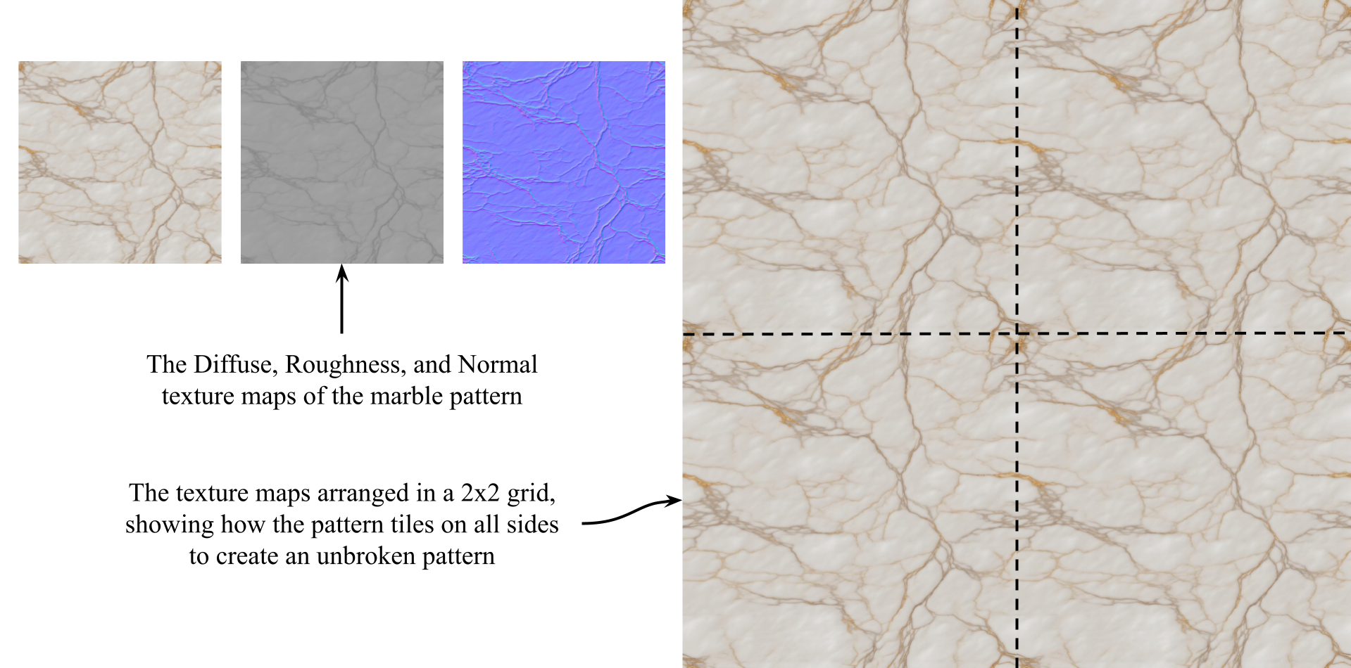
Figure 7:The AI generated, seamless marble texture on the Floor.usda. Left are the individual image textures, right is the texture repeated four times in a 2x2 grid.
The approach we’ve presented here is just one way we can begin to incorporate AI into the scene creation workflow. We have used it to demonstrate the key features of automating the process using cloud based resources, good prompt engineering, and Python. There will be other ways to reach the same goal, for instance, it has recently become possible to show a texture image to GPT-4o and ask it to convert it to a different texture type. GPT-4o then refers the image to DALL-E-3, and returns the requested texture map maintaining accurate detail. Unfortunately, at the time of writing, this capability is not available via API or inference endpoints, so we were unable to automate with Python here.
The techniques for automating communication with AI models that we have presented above will also be applicable for generating other types of content relevant to OpenUSD, such as 3D meshes or 360° environment textures. You simply need to find the models capable of creating what you need. Many of these things can also be done manually via web-based GUIs, or by running software locally if you have the necessary hardware. However, in this chapter we have confined our narrative to automating the process using Python. We have provided a selection of external resources in Appendix D to help you discover these services and encourage further exploration.
Remember, AI generation is a fast evolving medium, and whilst the assets we can produce today are only suitable in some settings, we are likely to see very high quality assets being created this way in the near future.
As we begin to grow our libraries of AI-generated 3D assets the challenge of managing them effectively starts to mirror the demands faced by entire industries. Whether in gaming, visual effects, product design, or virtual retail, organizing and retrieving assets at scale is essential, and vector databases are emerging as a key solution. We’ll explore them next.
10.4 Managing 3D Assets with Vector Databases
As the volume of 3D assets continues to grow in industries like gaming, AR/VR, and digital twins, efficiently organizing and retrieving these assets becomes a major challenge. Traditional approaches, such as folder hierarchies or manual keyword tagging, struggle to scale and often fail to capture the deeper meaning or context of assets.
AI offers a more powerful alternative through semantic search, a technique that interprets natural language and compares the underlying meaning rather than relying on exact keyword matches. This capability relies on transforming text descriptions into high-dimensional vectors, numerical representations encoding semantic features. An Embedding Model, such as OpenAI’s text-embedding-3-small, performs this transformation. These models, which can be machine learning models or cloud-based services, convert input data (typically text) into these meaning-rich embeddings. The resulting vectors are then stored in a vector database, enabling rapid comparison of meaning across extensive datasets.
Vector databases and semantic searches allow for highly precise and context-aware retrieval of assets, making them ideal for applications like recommendation systems, knowledge bases, or content discovery, where both relevance and specific criteria matter.
Semantic search allows users to describe what they are looking for in plain language, specifying aspects like an asset’s appearance, function, or context. The embedding model then converts this natural language query into a vector. This vector is used to retrieve results from the vector database whose own vectors indicate conceptual similarity to the query. Figure 8 illustrates this data flow: original model descriptors are converted by the embedding model and stored in the vector database, enabling subsequent queries to be converted and compared for the retrieval of similar assets.
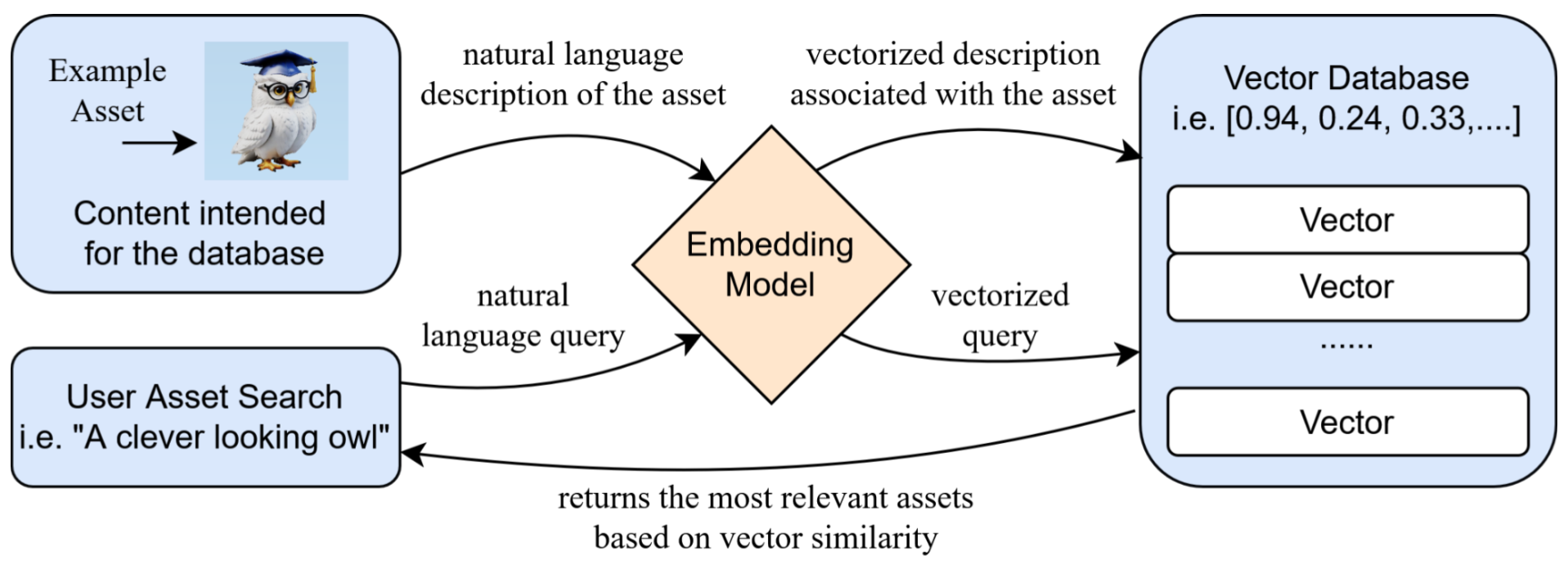
Figure 8:Illustrating the process of using a vector database for 3D asset management and retrieval. The description of a 3D asset is embedded into a high-dimensional vector and stored in the database. When a user generates a search query, it is also converted into an embedded vector. By comparing the similarity between the query vector and the vectors in the database, the system retrieves the most relevant assets, enabling efficient and intuitive search capabilities.
Vector databases are often used for online 3D asset search services, offering a significant advantage for creators and developers in fast-paced industries. While OpenUSD support isn’t yet universal in these databases, its increasing adoption by vendors and creators ensures growing compatibility with modern workflows. As OpenUSD expands, users can anticipate even wider support, simplifying the integration of purchased assets into USD-based pipelines. Appendix D provides helpful external resources for this.
It is also possible to build our own vector database, so let’s try it out. To practise building an example database we have collected four models from NVIDIA’s SimReady asset collections, and stored them on our GitHub repo. You can find them in the directory “Ch09/NVIDIA_Assets”. (For efficiency, we have not included the textures, or physics materials with these models, as we are only using them to demonstrate this retrieval technique). For those interested in exploring the full range of assets and building their own projects, we recommend visiting the NVIDIA Omniverse website to review the licensing terms and gain access to the complete asset library. The list of downloadable asset packs begins a quarter of the way down this page: https://
To demonstrate the creation and use of a vector database, let’s create a small example database, learn how to encode text descriptions, and store them as vectors. Once built we’ll demonstrate how to input a descriptive sentence, and retrieve the most relevant 3D model.
We’re going to be using an open source, high-speed vector database called Milvus (https://
- Work in Google Colab: (Simple) This is by far the easiest option, as the environments provided by Google Colab run on the Ubuntu distribution of Linux. For those readers who are not already using Colab, please refer to the section Appendix A.3.2, which will guide you on how to use a Colab notebook. If you’re already familiar with Colab, or just want to dive straight in, then simply create a new notebook here: https://colab.new/ and proceed with the code below.
- Install the Ubuntu subsystem via WSL: (Advanced) This option lets you run a Linux environment directly on Windows and will run Pymilvus locally. (https://
learn .microsoft .com /en -us /windows /wsl /install) - Connect to a cloud-based Milvus instance using Zilliz: (Advanced) Zilliz is a company that provides vector databases, like the open-source Milvus, to power AI applications. (https://zilliz.com/).
Next, let’s start the Python interpreter (not necessary if using Colab) and import the necessary library from pymilvus:
from pymilvus import MilvusClientTo enable semantic search, let’s first create a local Milvus database by initializing a MilvusClient with the file path ./milvus_demo.db, which stores the data on disk. Then we’ll define a collection named “demo_collection” using create_collection. This collection will hold the vector data, and we’ll specify a dimension of 1536, meaning that each vector contains 1,536 floating-point values that encode the semantic meaning of a text description. This dimension must match the size of the vectors produced by OpenAI’s text-embedding-3-small model to ensure Milvus can store and index the data correctly for similarity search:
# Initialize a Milvus client named "milvus_demo.db" in your working directory
milvus_client = MilvusClient("./milvus_demo.db")

# Create and define the collection name and dimension
milvus_client.create_collection(
    collection_name="demo_collection",
    dimension=1536
)
Now, let’s define the assets we’ll work with and create download URLs for each one. The link variable stores the base URL of the asset folder (in this case its our GitHub repository). The asset_names list contains the filenames of four example USD assets. Finally, asset_links uses a list comprehension to combine the base URL with each filename, producing a list of direct links to the asset files for later reference or download:
# Define the base URL of the asset folder
link = "https://github.com/learn-usd/learn-usd.github.io/tree/main/code_and_assets/Ch10/NVIDIA_Assets"

# Create a list of file names for the assets
asset_names = ["RackSmallEmpty_A1.usd", "RackLongEmpty_A1.usd", "WoodenCrate_A1.usd", "MetalFencing_A2.usd"]

# Produce a list of asset urls
asset_links = [link + asset_name for asset_name in asset_names]
Next, let’s define a list of natural language descriptions for each asset. The docs list contains concise phrases that describe the appearance or function of each asset. These descriptions will be used as input to the embedding model, which converts them into vectors for semantic search. Each description should clearly convey the asset’s purpose or characteristics to ensure meaningful results during retrieval:
docs = [
    "A small, empty storage rack",
    "A long and large empty storage rack",
    "A wooden crate for storage or transport.",
    "A section of metal fencing for barriers or enclosures.",
]
Be aware that the order of the assets in the list is important because the docs list (text descriptions) and the asset_links list (URLs) are aligned by index. When generating embeddings and later inserting data into Milvus, the script uses the same index (i) to match the vector (vectors[i]), the description (docs[i]), and the link (asset_links[i]). If the order of any of these lists changes independently, the vectors will no longer correctly correspond to the right assets or descriptions, which would corrupt the search results. Always ensure these lists stay aligned during editing or expansion.
Now, let’s use OpenAI’s API, and define a function to convert our text descriptions into vector embeddings using the text-embedding-3-small model. The get_openai_embedding function takes our text strings as input and returns the resulting embedding vector with return response.data[0].embedding. The final line calls this function for each item in the docs list, and stores the resulting list of vectors in the vectors variable. These embeddings will later be inserted into the Milvus vector database to support semantic search:
from openai import OpenAI

client = OpenAI(api_key="<your_openai_api_key_here>")

def get_openai_embedding(text):
    # Send the input text to the OpenAI API for embedding
    response = client.embeddings.create(
        input=text,
        # Specify the embedding model to use
        model="text-embedding-3-small"
    )
    # Extract and return the embedding vector from the API response
    return response.data[0].embedding

# Generate an embedding for each asset description and store in a list
vectors = [get_openai_embedding(doc) for doc in docs]
Now, we’re ready to put our data into the Milvus database. First we’ll construct a list of dictionaries—each dictionary represents an asset and includes four fields: a unique id, the asset’s embedding vector, its descriptive text, and the direct link to the asset file. These elements are combined using a list comprehension that loops through the indices of the vectors list. Then we’ll insert this structured list into the demo_collection in Milvus, making the data available for semantic search:
# Iterate over all assets to construct dictionaries for each asset
data = [{"id": i, "vector": vectors[i], "text": docs[i], "link": asset_links[i]} for i in range(len(vectors))]

# Insert the compiled data into the Milvus collection
milvus_client.insert(collection_name="demo_collection", data=data)
The code above should return “{‘insert_count’: 4, ‘ids’: [0, 1, 2, 3], ‘cost’: 0}”, which means:
- insert_count: 4: Milvus successfully inserted 4 records into the collection.
- ids: [0, 1, 2, 3]: These are the unique IDs assigned to the inserted records. They match the id values you provided in your data.
- cost: 0: The operation completed with negligible time cost (reported as 0 seconds).
We now have a vector database populated with semantically meaningful embeddings, and it’s ready to be queried using natural language inputs. The first step is to convert the natural language query into a vector, ready for comparison with the database’s vectors.
In each of the following two queries the first line defines a query string that describes a possible asset that we’re searching for, and the second line passes this text into the get_openai_embedding() function, which uses the embedding model to transform the text into a high-dimensional vector (embedding1) capturing its semantic meaning. These vectors will later be used to query the Milvus database for the most semantically similar assets:
# Defines a natural language search query
search_text1 = "An object that separates different areas"

# Converts the query into a semantic vector using OpenAI's embedding model via the previously defined function
embedding1 = get_openai_embedding(search_text1)

search_text2 = "A compact container"
embedding2 = get_openai_embedding(search_text2)
Having vectorized our queries let’s run a semantic search on the “demo_collection”. The following snippet sends our two query vectors (embedding1, and embedding2) to the collection. The limit=1 argument ensures that only the single closest match is returned for each query. The output_fields=[“text”, “link”] specifies that the results should include the original asset description (text) and its associated URL (link). The results will include metadata and similarity scores indicating how closely each result matches the input query:
result = milvus_client.search(
    collection_name="demo_collection",    # Name of the collection to search in
    data=[embedding1, embedding2],         # List of query vectors generated from user text
    limit=1,                              # Return only the top match for each query
    output_fields=["text", "link"]        # Include original asset description and download URL in results
)

print(result)    # Print the results
The result will be:
AI Response Begin [OpenAI text-embedding-3-small]

data: [[{'id': 3, 'distance': 0.40038830041885376, 'entity': {'text': 'A section of metal fencing for barriers or enclosures.', 'link': 'https://github.com/learn-usd/learn-usd.github.io/tree/main/code_and_assets/Ch10/NVIDIA_Assets/MetalFencing_A2.usd'}}], [{'id': 0, 'distance': 0.5244041681289673, 'entity': {'text': 'A small, empty storage rack', 'link': 'https://github.com/learn-usd/learn-usd.github.io/tree/main/code_and_assets/Ch10/NVIDIA_Assets/RackSmallEmpty_A1.usd'}}]]

AI Response End [blank line]
The query result from Milvus returns items ranked by semantic relevance to the search query. Each item in the result includes an id, a distance (a measure of similarity, where lower values indicate closer matches), and an entity containing the original description given to the matched asset, and a download link. For instance, for our first search query, ‘An object that separates different areas’, the top result is a metal fencing asset which has a distance of 0.40, showing it’s the best match.
You now have a working example of how to create a vector database and use it to perform semantic searches over asset metadata. While scaling this process to larger datasets would require more setup time, the long-term benefits are substantial. Semantic search powered by vector embeddings represent a significant advancement in data retrieval systems, and offer a powerful alternative to traditional keyword search by understanding the meaning behind queries even if exact terms don’t match. In practice, this approach unlocks faster, more intuitive access to large asset libraries, making it a valuable tool for any workflow involving complex digital content.
10.5 Unlocking the Future of AI for OpenUSD Workflows
Throughout this chapter, we’ve explored key ways in which AI can enhance OpenUSD workflows, but this is just the beginning. Beyond the foundational applications we’ve covered, there are vast opportunities for AI to push the boundaries of OpenUSD, particularly in fields like physics simulations, design optimization, and real-time content generation.
In design, AI tools like NVIDIA Physics-NeMo and nTop are transforming industries such as architecture and manufacturing by enabling rapid iteration and optimization of complex models. Combined with OpenUSD, these tools can streamline design processes and improve performance predictions.
In entertainment, gaming, and VR, AI-driven procedural content generation and intelligent agents will create richer, more dynamic experiences. Integrated with OpenUSD, this will allow for interactive environments that adapt to user actions and environmental changes.
AI will also enhance asset management in OpenUSD by automating tasks like tagging, categorizing, and optimizing scenes leading to more efficient workflows and better collaboration across industries.
The future of AI in OpenUSD workflows is just beginning, and as these technologies evolve, they will unlock even more opportunities for automation, design innovation, and creative expression. Together with Python scripting, the potential for revolutionizing how we create and interact with 3D environments is limitless.
Summary
- LLMs streamline the process of modifying OpenUSD scenes by enabling intuitive, natural language commands. Users can make real-time adjustments to scene elements without needing extensive coding knowledge.
- The OpenAI SDK provides the tools and libraries necessary to interact with AI models programmatically.
- To access AI models from platforms like OpenAI, NVIDIA NIM, and Hugging Face you’ll need an API key. This unique identifier authenticates your requests, ensuring only authorized users can utilize the models and services. This protects your data and resources from unauthorized access and misuse.
- An API request to an LLM typically includes a model parameter to choose the model, and a messages parameter, a list of dictionaries representing the conversation. Each dictionary contains a role (e.g., “user”, “assistant”, or “system”) and content, which holds the message text.
- A system message at the start of a conversation sets the LLM’s role and behavior, helping it generate more relevant responses. For example: “You are a helper for coding using Python for OpenUSD.”
- To extract specific elements from an AI’s response—such as Python or USD code, you can use Python’s regular expression (regex) module to target the content within code blocks.
- Due to the human-readable format of .usda files, LLMs can parse and understand them, facilitating tasks like generating and interpreting commands, implementing modifications, and providing content-based insights.
- Generative AI is capable of creating image textures, and 3D models. Though currently the standard of these is insufficient for professional studios, they can be useful for prototyping or less demanding scenarios.
- In image generation, LoRAs (Low-Rank Adaptation models) work by influencing a model’s output towards a particular style or content and require a trigger phrase to activate their effect.
- Vector databases use AI embedding models to encode natural language descriptions and search queries into high-dimensional vectors, enabling fast, precise, and context-aware retrieval of assets based on semantic similarity.