This chapter covers
- Generating a new USD scene with randomized objects
- Fine-tune placement behavior with customizable scatter controls
- Create a reusable, modular Blender add-on that bridges Blender and USD workflows
In this final chapter, we bring together the core ideas explored throughout the book — from constructing and transforming USD scenes, to working with geometry, animation, physics, and automation. The goal is to build a complete, functional Blender add-on that allows users to scatter USD assets — like rocks or trees — across a terrain with artistic control and physical realism. You’ll learn how to expose Python-powered scattering logic through Blender’s UI, giving artists the ability to choose assets, adjust distribution weights, control spacing, and export a USD scene — all without writing code.
This chapter is both a technical synthesis and a practical milestone. It shows how OpenUSD and Python can integrate cleanly into artist workflows, and how automation can amplify creativity in large-scale 3D environments.
By the end, you’ll have built a usable tool, sharpened your understanding of USD and Blender integration, and closed the loop from low-level scene manipulation to real-world pipeline applications.
12.1 A Minimal Toy Example: Scattering Cubes on a Math-Generated Plane
Before introducing complex terrain or USD stage composition, we start with a self-contained, minimal example. This toy setup will create a wavy plane from scratch using a simple math function and scatter cubes across its surface. The goal is to help you understand the essentials without the overhead of loading real assets.
First thing first, set ‘Ch12’ downloaded from https://
import os
new_directory = "<'/your/path/to/Ch12'>"
os.chdir(new_directory)
12.1.1 Create a Math-Generated Wavy Plane
To create a wavy plane, we’ll build on the flat grid example from Chapter 4. Previously, we created a simple 2D plane with four points. Now, we’ll enhance that by adding more points and a height function to turn the flat surface into a 3D wavy mesh.
Let’s start by setting up the USD stage and defining a mesh.
# Import the core USD and geometry modules
from pxr import Usd, UsdGeom

# Set the upward axis as y (common in Blender)
stage = Usd.Stage.CreateNew("wavy_plane.usda")
UsdGeom.SetStageUpAxis(stage, UsdGeom.Tokens.y)

# Define a mesh named 'plane' within the '/World' scope
wavy_plane = UsdGeom.Mesh.Define(stage, "/World/wavy_plane")
Next, we define the size of the plane, the resolution of the grid, and a height function that generates the wavy surface. size parameter defines the ranges for X and Y axes from -size to +size. resolution parameter controls how many points are sampled along each axis of the plane (X and Y). Think of it like pixel resolution in an image: A low resolution means fewer points are generated, and the plane will look jagged; A high resolution means more points are sampled, and the surface appears smoother and more detailed.
import math

# The plane spans from -size to +size along both X and Y axes.
# In this case, the plane covers a 20×20 unit area
size = 10

# Resolution defines how many points we sample in each axis
resolution = 50

# Function that defines elevation (Z) based on X and Y
def get_height(x, y):
    return math.sin(0.5 * x) * math.cos(0.5 * y)
Now we loop over a resolution x resolution grid to generate points for the terrain surface:
# Initialize an empty list of 3D points
points = []

# Loop over grid coordinates in X and Y axis
for x in range(resolution):
    for y in range(resolution):
        # Normalize x and y to [-size, +size], mapping from pixel to real-world units
        xf = (x / (resolution - 1)) * (2 * size) - size
        yf = (y / (resolution - 1)) * (2 * size) - size

        # Compute the Z (height) using our math function
        z = get_height(xf, yf)

        # Store the 3D point
        points.append((xf, yf, z))
We’ve computed the (x, y, z) coordinates for each vertex in our wavy plane, the next step is to connect those vertices into faces. Since we want a mesh made of quads (rectangles made of 4 points), we define each face using 4 vertex indices.
# Stores all the vertex indices that define each face (in groups of 4)
faceVertexIndices = []

# Holds the number of vertices per face. Since we’re creating quads, this will always be 4
faceVertexCounts = []

# Loop through the grid cells, skipping the last row and column to avoid indexing out of bounds
for x in range(resolution - 1):
    for y in range(resolution - 1):
        # Compute the indices of the four corners of each quad
        i0 = x * resolution + y
        i1 = i0 + 1
        i2 = i0 + resolution + 1
        i3 = i0 + resolution

        # Add the four vertex indices that make up one quad to the master index list
        faceVertexIndices.extend([i0, i1, i2, i3])

        # Append the value 4 to indicate that this face uses 4 vertices
        faceVertexCounts.append(4)
Finally we plug in all the data above to a UsdGeom.Mesh so that our wavy plane becomes a proper USD geometry.
# Sets the vertex positions into the points attribute of the mesh
wavy_plane.GetPointsAttr().Set(points)

# Assigns how many vertices make up each face — in our case, all are 4 for quads
wavy_plane.GetFaceVertexCountsAttr().Set(faceVertexCounts)

# Specifies the exact vertex indices for each face
wavy_plane.GetFaceVertexIndicesAttr().Set(faceVertexIndices)

# Save the stage
stage.Save()
Let’s check the created wavy plane in blender, and you will see a smooth wavy plane as in Figure 1.
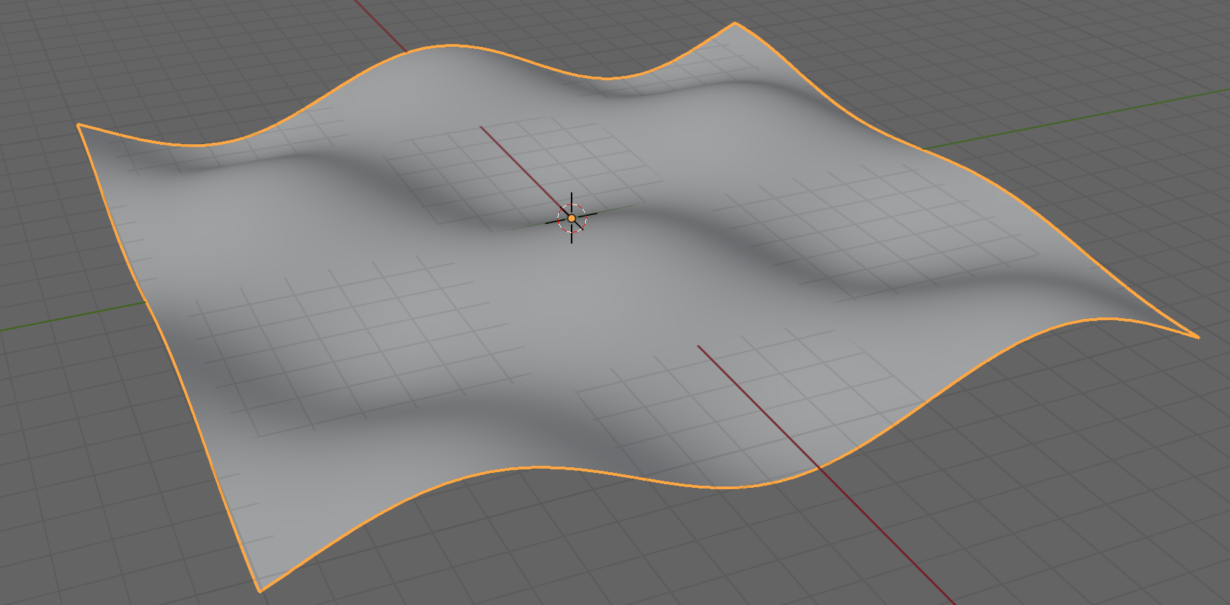
Figure 1:A wavy plane generated by a math function.
12.1.2 Scatter Cubes on the Wavy Plane
We will now scatter cubes randomly across the wavy terrain using USD’s highly efficient PointInstancer. If you recall from Chapter 8, we used PointInstancer to build a forest scene, where 20 tree instances were handled gracefully with minimal memory overhead. The same principle applies here: rather than duplicating geometry, we define a single cube prototype and reference it many times at different locations. In this section, we’ll walk through a similar process, starting with defining the cube prototype.
# Define the path in the USD stage where the cube prototype will be placed
proto_cube_path = "/World/Prototypes/Cube"

# Create a Cube geometry at the specified path
cube = UsdGeom.Cube.Define(stage, proto_cube_path)

# Set the size of the cube to 0.3 units
cube.CreateSizeAttr().Set(0.3)
Next, we generate random positions for our cube instances using Python’s built-in random module, similar to what we did in Chapter 08. The key difference here is that we need to place the cubes on top of the wavy terrain, so for each sampled (x, y) position, we compute the corresponding z value using our earlier get_height function. This ensures the cubes sit directly on the surface of the generated plane.
# Import random module, which is pre-installed with Python
import random

# Set how many cube instances we want to scatter
num_instances = 100

# A list to hold the generated 3D positions of each instance
positions = []

# A list to store prototype indices — each value points to a prototype in the instancer
proto_indices = []


# Loop to generate a random (x, y) pair for each instance
for _ in range(num_instances):
    # Randomly sample X and Y within the bounds (-size, size) of the plane
    x = random.uniform(-size, size)
    y = random.uniform(-size, size)

    # Determine the z-axis value at that point
    z = get_height(x, y)

    # Append the position for each cube
    positions.append(Gf.Vec3f(x, y, z))

    # Append each instance’s cube prototype index 0
    proto_indices.append(0)
Finally, let’s assign positions and indices to PointInstancer.
# Define the PointInstancer prim
instancer = UsdGeom.PointInstancer.Define(stage, "/World/Instancer")

# Set the prototype asset references to the PointInstancer
instancer.CreatePrototypesRel().SetTargets([proto_cube_path])

# Assign the list of positions to place the cubes
instancer.CreatePositionsAttr().Set(positions)

# Specify which prototype each instance uses (here all 0)
instancer.CreateProtoIndicesAttr().Set(proto_indices)

# Save the stage
stage.Save()
You should see results similar to those shown in Figure 2. Keep in mind that because the cube positions are generated randomly, your scene may not look identical, but the overall effect should be comparable: cubes scattered naturally across the wavy surface.
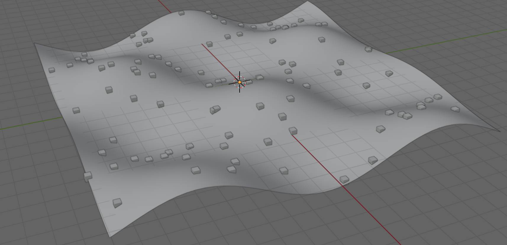
Figure 2:A wavy plane with randomly scattered cubes.
Now that we’ve successfully used PointInstancer to place simple cubes on a mathematically defined terrain, let’s take it a step further—replacing these primitives with more complex assets, and introducing additional controls like prototype weights and minimum distances between instances.
12.2 Complex Real Assets and additional controls
In real-world scenarios, we typically work with existing terrain assets rather than generating them from mathematical functions. These assets often have complex, irregular geometry, and there’s no simple equation we can use to compute surface height. To extend the toy example above into something production-ready, we’ll need to tackle several practical challenges:
- Determine the terrain’s XY boundary — so we know the valid region from which to sample points.
- Query the surface height (Z value) for a given (X, Y) location — to correctly place objects on top of the terrain geometry.
- Enforce minimum spacing — to prevent scattered objects from overlapping.
- Introduce visual variety — by adding randomization in scale and rotation of each instance.
We’ll walk through each of these enhancements step-by-step as we move from scattering simple cubes to placing detailed rock assets on a real terrain model.
12.2.1 Preparing the Terrain for Placement
To work with a real terrain asset, we’ll need to extract its geometry, measure its bounds, and perform queries on its surface points. These are structured as reusable helper functions, making the main logic cleaner and more modular.
Let’s start by identifying the first usable mesh under a given prim path. This function searches for the first UsdGeom.Mesh within the given prim hierarchy and returns both the mesh object and its vertex points. The key idea is using Usd.PrimRange to walk through a prim and everything inside it, so we can find mesh objects even if they’re hidden deep under other groups or transforms. It’s essential for working with asset files that might include groups, transforms, or references.
def get_first_mesh_and_points(stage, prim_path):
    # Get the prim located at prim_path
    root_prim = stage.GetPrimAtPath(prim_path)

    # Check whether the prim exists and is valid:
    # If the path is invalid or the prim is missing, return early with a warning
    if not root_prim or not root_prim.IsValid():
        print(f"Invalid prim at path: {prim_path}")
        return None, None

    # Traverse the subtree rooted at root_prim using Usd.PrimRange
    for prim in Usd.PrimRange(root_prim):
        # For each prim in the hierarchy, check whether it is a UsdGeom.Mesh
        if prim.IsA(UsdGeom.Mesh):
            # Cast the prim to a UsdGeom.Mesh
            mesh = UsdGeom.Mesh(prim)
            # Retrieve the list of points from the mesh’s points attribute
            points = mesh.GetPointsAttr().Get()
            # Return the first mesh along with its points
            return mesh, points

    # If no mesh was found after searching the prim and its descendants, print a message and return None.
    print(f"No UsdGeom.Mesh found under {prim_path}")
    return None, None
Program 1:Get the First Mesh and Its Points
Once we have the mesh, we compute its spatial extent. Recall that in Chapter 6, we already created a function to get the bounding box for a given prim. Here we will add the overall size of the prim as additional output. It helps set a lower bound for the minimum distance between scattered assets — typically equal to or slightly larger than the largest asset’s footprint.
def compute_bounding_box(stage, prim_path):
    prim = stage.GetPrimAtPath(prim_path)
    purposes = [UsdGeom.Tokens.default_]
    bboxcache = UsdGeom.BBoxCache(Usd.TimeCode.Default(), purposes)
    bboxes = bboxcache.ComputeWorldBound(prim)
    min_point = bboxes.ComputeAlignedRange().GetMin()
    max_point = bboxes.ComputeAlignedRange().GetMax()
    size = max_point - min_point
    return min_point, max_point, size
Program 2:Compute the Bounding Box .
Then, to correctly position an asset on the surface, we need to know its elevation (z-value) for a given (x, y). We define a helper function that takes a 2D query point (x, y) and returns the index of the closest vertex in the terrain mesh. It does nearest-neighbor lookup without requiring external libraries but only requires import numpy as np. By using the z-value from that nearest vertex, we can “snap” each scattered asset directly onto the terrain.
def find_nearest_index(data_points, query_point):
    # data_points contains X and Y dimensions of each point of the terrain.
    # query_point is the point we want to place on the terrain, i.e. the sampled points.

    # Compute the Euclidean distance between the query_point and each point in data_points.
    distances = np.linalg.norm(data_points - query_point, axis=1)

    # Find the index of the point with the smallest distance to the query point.
    return np.argmin(distances)
Program 3:Find the Nearest Index
Finally, to avoid overlapping placements, we introduce a distance-checking function. It verifies that a new placement is far enough from all previously placed positions, helping maintain realism and avoiding collisions.
def is_far_enough(x, y, placed_positions, min_dist):
    # (x, y) is the new point we want to check whether it is far enough
    # from the previously placed points placed_positions, based on min_dist.

    # Loop through each point (px, py) already accepted in placed_positions
    for px, py in placed_positions:
        # Compute squared Euclidean distance between new point and existing point
        if (x - px)**2 + (y - py)**2 < min_dist**2:
            # If any previous point is too close, reject this position
            return False

    # If no conflicts found, accept this point
    return True
Program 4:Check Distance
12.2.2 Putting It All Together: run_usd_scatter()
Now that we’ve built a set of helper functions to extract mesh data, compute terrain bounds, query surface height, and enforce spacing between instances, it’s time to bring everything together into a single reusable function: run_usd_scatter.
This function serves as the core engine of our scattering pipeline. It takes in a terrain asset, a list of prototype objects, and several user-defined parameters such as the number of instances, minimum spacing, and optional placement bounds. It then outputs a complete USD stage where instances are scattered intelligently across the terrain surface. Let’s walk through the parameters first, then explore the function step by step.
from pxr import Usd, UsdGeom, Gf, Vt
import random
import numpy as np

def run_usd_scatter(
    output_path,           # B: The path to the USDA file where the final scattered scene will be saved
    terrain_asset_path,    # C: The file path to the USDA file containing the terrain mesh
    terrain_prim_path,     # D: The prim path for the terrain
    prototypes,            # E: Defines the properties for prototype objects to scatter
    num_instances,         # F: The total number of instances to place across the terrain surface
    min_distance=None,     # G: Optional parameter. Minimum allowed distance between any two scattered objects
    bounds=None,           # H: Optional parameter. The max distance from origin (0,0) on the X/Y plane where objects can be placed
):
    # Function implementation goes here
Program 5:run_usd_scatter
The prototypes parameter contains properties for each object to scatter: “file” specifies the path to the USD asset file, “path” indicates the prim path within that file, and “weight” defines the relative selection weight used during random sampling.
The min_distance is an optional parameter that helps avoid overlapping or collisions. If not specified, it will be estimated from prototype sizes.
The bounds is an optional parameter that sets the maximum distance from the origin (0, 0) on the X/Y plane where objects can be placed. Objects will be scattered within the square region [-bounds, +bounds], with a margin equal to min_distance automatically subtracted to prevent objects from being clipped at the edge. If not specified, bounds are inferred from the terrain’s bounding box.
Let’s start with creating a new USD stage where we’ll assemble the scattered scene. We also reference the terrain asset, which acts as the base surface for object placement.
    # Create a new USD stage and specify the output_path where the result will be saved
    stage = Usd.Stage.CreateNew(output_path)

    # Set the up axis of the scene to Z
    UsdGeom.SetStageUpAxis(stage, UsdGeom.Tokens.z)

    # Define a new transform prim at the location where the terrain will be referenced
    terrain_ref = UsdGeom.Xform.Define(stage, terrain_prim_path)

    # Add a reference to the external terrain asset file saved at terrain_asset_path
    terrain_ref.GetPrim().GetReferences().AddReference(terrain_asset_path)
Program 6:Stage Initialization and Asset Loading
Once the terrain asset is loaded into the stage, the next step is to extract its geometry and compute relevant spatial properties with helper functions defined earlier. We’ll use this data to determine where it’s safe and reasonable to scatter objects.
    # Use get_first_mesh_and_points to retrieve the first mesh and its vertex points from the terrain prim
    terrain_mesh, terrain_points = get_first_mesh_and_points(stage, terrain_prim_path)

    # Compute the bounding box of the terrain mesh using compute_bounding_box
    min_point, max_point, _ = compute_bounding_box(stage, terrain_mesh.GetPath())

    # Convert the terrain’s point list into a NumPy array to enable efficient vector math
    terrain_points_arr = np.asarray(terrain_points)

    # Extract the X and Y coordinates from each vertex
    terrain_points_arr_xy = np.asarray(terrain_points_arr)[:, :2]
Program 7:Terrain Mesh Data and Properties
Notice that on the last line, we extract just the X and Y coordinates from each vertex. Since we sample positions in 2D and look up the height (Z) later, this 2D slice is all we need for spatial sampling.
Next, we handle the case where bounds was not explicitly provided by the user:
    if bounds is None:
        # Convert the bounding box corners to NumPy arrays and extract only the X and Y dimensions
        min_point_arr_xy = np.asarray(min_point)[:2]
        max_point_arr_xy = np.asarray(max_point)[:2]

        # Compute the smallest (absolute) distance to the edge along X or Y
        bounds = float(np.min(abs(np.concatenate((min_point_arr_xy, max_point_arr_xy)))))
Program 8:Calculate Bounds on Terrain
Then we move on to prepare the prototype objects that will be scattered across the terrain. Each prototype is defined by a USD asset file, a stage path, and a sampling weight. We store their paths, compute their sizes, and estimate spacing constraints based on their bounding boxes.
    # List of all prim paths where prototype objects will be defined in the USD stage
    proto_paths = []

    # Corresponding list of weights used to control random selection during scattering
    proto_weights = []

    # Stores the size of each prototype, which is used to estimate safe placement distance
    proto_size_list = []

    for proto in prototypes:
        # Record the prim path where this prototype will be instanced from each proto in prototypes
        proto_paths.append(proto["path"])

        # Store the prototype’s weight for use in weighted random selection
        proto_weights.append(proto["weight"])

        # Define an empty Xform prim at the specified path in the stage. This is the anchor where the asset will be referenced
        prim = stage.DefinePrim(proto["path"], "Xform")

        # Add a reference to the prototype’s USD file, bringing the actual geometry into the stage
        prim.GetReferences().AddReference(proto["file"])

        # Find the first mesh inside the referenced asset
        proto_mesh, _ = get_first_mesh_and_points(stage, proto["path"])

        # Compute the prototype’s bounding box to estimate its size
        _, _, proto_size = compute_bounding_box(stage, proto_mesh.GetPath())

        # Extract the maximum extent in X or Y to represent its size. This will be used to calculate spacing
        proto_size_list.append(np.max(proto_size[:2]))

    # If the user hasn’t provided a min_distance, we compute one automatically
    if min_distance is None:
        # Use the largest prototype size as the default minimum distance between instances
        min_distance = float(max(proto_size_list))

    # Adjusts the placement boundary to create a margin
    real_bounds = max(0.0, bounds - min_distance/2)
Program 9:Prototypes Setup
After setting up the terrain and prototypes, we move on to the scattering logic. Compared to the earlier toy example, this version adds a minimum distance check, computes the Z value based on each (X, Y) position, and applies random rotation around the Z-axis — making it suitable for more complex, real-world scenarios.
    # Initialize a list to track all accepted (x, y) positions, used to enforce minimum spacing between instances
    placed_positions = []

    # Initialize a list to track instance positions (x, y, z) where the prototypes will be placed (Gf.Vec3f)
    positions = []

    # Initialize a list of instance orientations (Gf.Quath)
    orientations = []

    # Initialize a list of instance scales (Gf.Vec3f)
    scales = []

    # Initialize a list of prototype indices
    indices = []


    # Main sampling loop: continues until the desired number of instances has been placed
    while len(positions) < num_instances:
        # Randomly sample a new candidate (x, y) position within the usable bounds of the terrain
        x = random.uniform(-real_bounds, real_bounds)
        y = random.uniform(-real_bounds, real_bounds)

        # Check that the candidate position is far enough from previously placed instances using the min_distance constraint
        if is_far_enough(x, y, placed_positions, min_distance):
            sample_point_xy = np.array([x, y])

            # Find the nearest point on the terrain surface and extract its Z value to place the object
            close_point_index = find_nearest_index(terrain_points_arr_xy, sample_point_xy)
            z = float(terrain_points_arr[close_point_index, 2])

            # Record the accepted position in both tracking lists
            placed_positions.append((x, y))
            positions.append(Gf.Vec3f(x, y, z))

            # Generate a random rotation around the Z axis and store it as a quaternion
            angle_deg = random.uniform(0, 360)
            rotation = Gf.Rotation(Gf.Vec3d(0, 0, 1), angle_deg)
            quat = rotation.GetQuat()
            orientations.append(Gf.Quath(quat))

            # Apply random uniform scaling to the object to create variation and store it
            scale = random.uniform(0.8, 1.2)
            scales.append(Gf.Vec3f(scale, scale, scale))

            # Randomly choose which prototype to use for this instance, based on the user-provided weights. Store the index
            index = random.choices(range(len(proto_paths)), weights=proto_weights)[0]
            indices.append(index)
Program 10:Scatter
After generating all the necessary instance attributes—positions, orientations, scales, and prototype indices—we now pass this data into a UsdGeom.PointInstancer. This is the final step that writes the instance configuration to the USD stage, and the process is similar to the previous toy example.
    # Create a new PointInstancer prim at /World/Instances
    instancer = UsdGeom.PointInstancer.Define(stage, "/World/Instances")

    # Set the list of prototype targets. Each item in proto_paths corresponds to a prototype prim that was referenced earlier in the stage
    instancer.CreatePrototypesRel().SetTargets(proto_paths)

    # Set the world-space position of each instance. Each value is a Gf.Vec3f coordinate derived from the terrain surface
    instancer.CreatePositionsAttr(Vt.Vec3fArray(positions))

    # Set the rotation of each instance, stored as quaternions (Gf.Quath)
    instancer.CreateOrientationsAttr(Vt.QuathArray(orientations))

    # Set the scale for each instance
    instancer.CreateScalesAttr(Vt.Vec3fArray(scales))

    # Set the prototype index for each instance
    instancer.CreateProtoIndicesAttr(Vt.IntArray(indices))


    # Save the USD stage
    stage.Save()
Program 11:Set Instancer Data
Now that we’ve defined the run_usd_scatter function, let’s try it out with provided assets under the ch11 folder (downloaded from GitHub: TODO). There we provided the terrain assets and three rock assets (under the “Assets” folder). After running the code below, you can check the final results under “shading” similar to Figure 3.
terrain_asset_path = "./Terrain.usda"
terrain_prim_path = "/World/Terrain"

prototypes = [
    {"path": "/World/Prototypes/Rock1", "file": "./Assets/Rock_1.usd", "weight": 0.5},
    {"path": "/World/Prototypes/Rock2", "file": "./Assets/Rock_2.usd", "weight": 0.3},
    {"path": "/World/Prototypes/Rock3", "file": "./Assets/Rock_3.usd", "weight": 0.2},
]

output_path = "scattered_rock.usda"
num_instances = 30

# Run the scattering process with optional bounds and min_distance set to None (will be computed automatically)
run_usd_scatter(output_path, terrain_asset_path, terrain_prim_path, prototypes, num_instances, bounds=None, min_distance=None)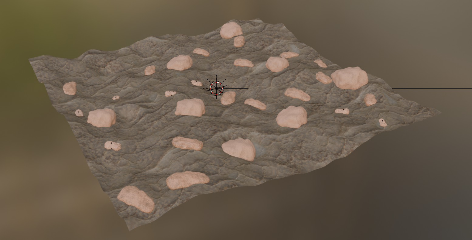
Figure 3:Scattered rocks on the terrain, generated using run_usd_scatter function.
Now that we’ve completed and tested our scattering logic with real terrain and assets, the final step is to make this functionality more accessible — especially for artists and non-programmers. Rather than requiring users to run Python scripts manually, we can wrap everything into a Blender add-on with a simple UI for loading terrain, selecting assets, adjusting parameters, and generating the scattered scene with one click. By the end, you’ll have a fully functional add-on that combines Python automation with artist-friendly controls — a practical and polished way to deliver OpenUSD tools in a creative workflow.
12.3 Blender Add-on
A Blender add-on is simply a Python package that extends Blender’s functionality. It gives you the power to create custom panels, operators, buttons, and even integrate external libraries all directly inside Blender’s UI.
Our goal is to turn the run_usd_scatter() function into an easy-to-use tool inside Blender’s sidebar. It incorporates the functionality to:
- Select terrain and prototype asset paths via file pickers
- Set parameters like number of instances, minimum distance, and sampling bounds
- Click a single button to generate the USD scene
Under the hood, a Blender add-on is simply a .zip file containing an init.py file, which defines the user interface and registers the add-on with Blender, along with any supporting Python scripts. In our case, the folder structure looks like this:
usd_scatter_addon/
├── __init__.py               # Blender UI and registration entry point
├── core/
│   ├── __init__.py           # Empty file, marking 'core' as a Python module
│   └── scatter.py            # Contains the run_usd_scatter function and helper utilities
“usd_scatter_addon/” is the root folder of the add-on. The top level init.py file defines the Blender UI to enable the add-on. “core/” is a subfolder that contains reusable backend logic, separate from Blender-specific code and helping organize and isolate core functionality. The second level init.py lives in “core/” is an empty file that indicates ‘core’ as a module. The scattering logic, i.e. run_usd_scatter and its helper functions, lives in core/scatter.py. It contains all the code, and we will not go over it again here. So let’s focus on the top level init.py file. At a high level, it is usually made up of the parts shown in Table 1.
Table 1:Components in __init__.py for Blender Add-on
| Property | Purpose |
|---|---|
bl_info | Record metadata so Blender can recognize and display the add-on |
PropertyGroups | Data models that store the user’s input |
Panel | The visual UI panel you see in Blender’s sidebar, where buttons and input fields go. |
Operators | The actions you run when clicking a button |
Register / Unregister | Functions that tell Blender how to load and clean up the add-on |
Now let’s map each of those parts to what we’re building in our USD object scatter add-on:
Blender components in the USD Object Scatter Add-on
| Blender Component | What It Does in This Add-on |
|---|---|
bl_info | Declares this as the USD Object Scatter tool. |
PrototypeItem | Represents one prototype rock or object (with file, path, weight). |
ScatterProperties | Holds all settings for the scattering task (output path, terrain, instance count, etc.). |
OBJECT_PT_usd_scatter | Creates a new UI panel in the Blender sidebar under “USD Scatter.” |
OBJECT_OT_add_prototype | Adds new prototype entries in the UI (e.g., Rock1, Rock2, Rock3). |
OBJECT_OT_run_usd_scatter | When the user clicks “Run USD Scatter,” this operator calls the actual Python logic to generate the USD stage. |
register() / unregister() | Hook all this into Blender so it appears when the add-on is enabled. |
Let’s start by setting the add-on metadata in bl_info. It is a dictionary containing add-on metadata such as the title, version and author to be displayed in the Preferences add-on list. It also specifies the minimum Blender version required to run the script.
bl_info = {
    # The name of the add-on as it appears in Blender’s Add-ons panel (Edit > Preferences > Add-ons)
    "name": "USD Object Scatter",

    # Author name
    "author": "Your Name",

    # The version number of add-on
    "version": (1, 0),

    # The minimum Blender version this add-on is compatible with
    "blender": (4, 2, 0),

    # The place in the UI for the add-on. In this case: inside the 3D Viewport’s Sidebar under a tab called USD Scatter
    "location": "View3D > Sidebar > USD Scatter",

    # Add-on description
    "description": "Scatter USD prototypes on terrain with options for weights, bounds, and min distance",

    # Determines where Blender files this add-on in the add-ons browser (e.g., Object, Import-Export, Animation). This affects how users find it.
    "category": "Object"
}
Program 12:bl_info
This metadata block is how Blender identifies and labels the add-on. It’s the first thing users see in the Preferences window, and it also determines where your add-on appears in the UI.
Now let’s move on to loading required python packages. Notice that you don’t need to install any extra packages, since bpy is Blender’s own Python API and always available inside Blender.
# Imports Blender’s Python API. It gives your add-on access to everything in Blender: UI elements, scene data, 3D objects, file paths, etc.
import bpy

# Load the types of input fields you can show in Blender’s UI
from bpy.props import StringProperty, FloatProperty, IntProperty, CollectionProperty, PointerProperty

# Load the building blocks of the Blender UI
from bpy.types import Panel, Operator, PropertyGroup


# This imports the main logic function — run_usd_scatter() — from the scatter.py file inside core/ folder
from .core.scatter import run_usd_scatter
Program 13:Load Packages
bpy.props is a module in Blender’s Python API that provides property types used to define custom UI input fields and data storage. These properties are commonly added to classes like PropertyGroup so they can appear in panels and store user input. Commonly used types are listed in Table 3.
Table 3:Input type for bpy.props
| Type | Purpose |
|---|---|
StringProperty | Text input (e.g., file paths) |
FloatProperty | Decimal numbers (e.g., scale, weight) |
IntProperty | Whole numbers (e.g., number of instances) |
CollectionProperty | A list of items (e.g., list of rock types) |
PointerProperty | A reference to another group of settings |
For bpy.types, it contains the base classes used to define custom UI elements and behavior, such as panels, operators, and property groups. When you create an add-on, you typically subclass from these types to integrate your code into Blender’s interface and event system.
Let’s begin by building the UI blocks. We need one group to collect user input for the objects to be scattered, and another for the overall scattering parameters. In Blender, this is done using PropertyGroup from bpy.types, which lets us bundle related properties into structured, reusable blocks.
We define the settings for each scatterable object using a class called PrototypeItem, which inherits from PropertyGroup. This acts as a reusable data container, holding the USD file path, prim path, and weight for each prototype.
# Defines a reusable “data block” for one scatterable item via PropertyGroup, will show up in Blender UI
class PrototypeItem(PropertyGroup):

    # Specifies the usd file path for the object to scatter
    usd_path: StringProperty(name="USD Path")

    # Specifies the prim path for the object to scatter
    stage_path: StringProperty(name="Stage Path")

    # Specifies the chance of the object appearing
    weight: FloatProperty(name="Weight", min=0.0)
Program 11:Defining a Prototype Object
Once we’ve defined what to scatter, we need to set the rules for how scattering works — like which terrain to use, how many items to place, and how far apart they should be. These settings are stored in the ScatterProperties class, which, like PrototypeItem, is a PropertyGroup that stores user input in a structured way.
# Defines input parameters for scattering, will show up in Blender UI
class ScatterProperties(PropertyGroup):

    # File path where the final output scene will be saved
    output_path: StringProperty(name="Output USDA Path")

    # File path for the terrain USDA file
    terrain_asset: StringProperty(name="Terrain USDA File")

    # The prim path within the terrain file. The default is "/World/Terrain"
    terrain_path: StringProperty(name="Terrain Prim Path", default="/World/Terrain")

    # Number of instances to place on the terrain
    num_instances: IntProperty(name="Number of Instances", default=20, min=1)

    # An optional spacing rule: prevents objects from being placed too close to one another
    min_distance: FloatProperty(name="Minimum Distance (optional)", default=0.0)

    # An optional XY boundary that limits how far from the center we can sample positions
    bounds: FloatProperty(name="XY Bound (optional)", default=0.0)

    # This connects the list of PrototypeItems defined earlier. Blender treats this as a dynamic, scrollable list in the UI.
    prototypes: CollectionProperty(type=PrototypeItem)
Program 15:Setting Up Scattering Parameters
After defining the necessary properties, the next step is to bring them into Blender’s interface so users can interact with them visually. This is done by creating a custom UI panel, which we define using the Panel class from bpy.types.
A Panel in Blender represents a section of the user interface — typically shown in the sidebar of the 3D Viewport. By subclassing bpy.types.Panel, we can specify where the panel appears, what it’s called, and what UI elements it contains. Inside the draw() function, we lay out the property fields we want to expose to the user, using the inputs we defined earlier in PropertyGroup.
In our case, we create a panel called OBJECT_PT_usd_scatter, which displays the output file path, terrain settings, prototype list, and action buttons like “Add Prototype” and “Run USD Scatter.” This panel serves as the front-end interface for our entire tool — turning backend logic into something intuitive and artist-friendly.
# Defines a new UI panel class in Blender. Panels control what the user sees in the sidebar
class OBJECT_PT_usd_scatter(Panel):

    # The title displayed at the top of the panel in the Blender UI
    bl_label = "USD Scatter"

    # A unique internal ID Blender uses to reference this panel. Convention is to prefix with OBJECT_PT_
    bl_idname = "OBJECT_PT_usd_scatter"

    # Specifies where this panel appears — here, in the 3D Viewport
    bl_space_type = 'VIEW_3D'

    # Specifies the region within the space — 'UI' means the sidebar
    bl_region_type = 'UI'

    # This places the panel under the “USD Scatter” tab in the sidebar, creating a dedicated tab for the tool
    bl_category = 'USD Scatter'

    # draw() function controls what appears in the UI when the panel is shown. Blender calls this automatically
    def draw(self, context):
        # layout is used to add buttons, text boxes, etc. to the panel
        layout = self.layout
        # Retrieves the user input values defined earlier in ScatterProperties. This is the data the panel will show and let users edit
        props = context.scene.scatter_props

        # Add labeled input boxes for each setting defined in ScatterProperties. Blender automatically generates a text field, number field, or slider depending on the property’s type
        layout.prop(props, "output_path")
        layout.prop(props, "terrain_asset")
        layout.prop(props, "terrain_path")
        layout.prop(props, "num_instances")
        layout.prop(props, "min_distance")
        layout.prop(props, "bounds")

        # Add a small label heading above the prototype list
        layout.label(text="Prototypes")

        # Loops through each prototype the user has added
        for proto in props.prototypes:

            # Creates a visual box for each prototype
            box = layout.box()

            # Adds input fields for each of the prototype’s properties: file path, prim path, and weight
            box.prop(proto, "usd_path")
            box.prop(proto, "stage_path")
            box.prop(proto, "weight")

        # Adds a button that lets users add another prototype to the list. It runs the operator OBJECT_OT_add_prototype (define later)
        layout.operator("object.add_prototype")

        # Adds a button that executes the scattering logic, calling the operator OBJECT_OT_run_usd_scatter (define later)
        layout.operator("object.run_usd_scatter")
Program 1:Panel Definition
Figure 4 shows a screenshot of the final UI, giving you a sense of how it comes together visually.
You may notice that some functions appear here before we’ve fully explained them — for instance, props = context.scene.scatter_props is used to access user input. We’ll see later how this connection is established through the register() function, which links custom properties to Blender’s internal data model.
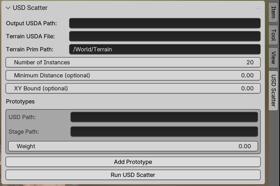
Figure 4:Blender UI for USD scatter.
With the panel now in place, we’ll turn to the logic behind the buttons — defined through two custom Operator classes. In Blender, operators are special classes that define actions, which are things that happen in response to user input, like clicking a button, executing a command, or performing a transformation. Operators are defined by subclassing bpy.types.Operator, and they typically contain an execute() method where the actual logic lives. Each operator is identified by a unique bl_idname, which is used to call it from buttons or menus, and a bl_label, which is the name shown in the UI. Once registered, these operators can be triggered from the interface, just like the buttons we created in the panel earlier. In our add-on, we define two operators:
- One to add a new prototype entry to the UI list
- One to run the scattering process using the current settings
Let’s look at the main operator first: the one that triggers the actual scattering function.
# Defines a new operator class to run the main scatter logic
class OBJECT_OT_run_usd_scatter(Operator):

    # The unique ID Blender uses to reference this operator. Used in the panel with layout.operator("object.run_usd_scatter")
    bl_idname = "object.run_usd_scatter"

    # The button label that appears in the UI panel
    bl_label = "Run USD Scatter"

    # execute() function is called when the button is clicked
    def execute(self, context):

        # Retrieves the user input values defined earlier in ScatterProperties
        props = context.scene.scatter_props

        # Prepares a list to hold all the prototype data in a format that run_usd_scatter expects
        prototypes = []

        # Loops through each user-defined prototype in the UI
        for p in props.prototypes:

            # Converts each prototype’s properties into a dictionary (with file, path, weight keys)
            prototypes.append({
                "file": p.usd_path,
                "path": p.stage_path,
                "weight": p.weight
            })

        # Calls the core function run_usd_scatter, passing in all the user inputs as arguments
        run_usd_scatter(
            output_path=props.output_path,
            terrain_asset_path=props.terrain_asset,
            terrain_prim_path=props.terrain_path,
            prototypes=prototypes,
            num_instances=props.num_instances,
            min_distance=props.min_distance if props.min_distance > 0 else None,
            bounds=props.bounds if props.bounds > 0 else None
        )

        # Signals to Blender that the operation completed successfully
        return {'FINISHED'}
Program 17:Operator – Running the Scatter Logic
Now let’s walk through the second operator, which is responsible for adding a new prototype entry to the UI. This one is simpler, but still crucial for making the UI dynamic and flexible.
# Defines a new operator class to add prototypes.
class OBJECT_OT_add_prototype(Operator):

    # The unique ID Blender uses to reference this operator. Used in the panel with layout.operator("object.add_prototype")
    bl_idname = "object.add_prototype"

    # The button label that appears in the UI panel
    bl_label = "Add Prototype"

    # execute() function is called when the button is clicked
    def execute(self, context):

        # Accesses the list of prototypes and adds a new, empty PrototypeItem
        context.scene.scatter_props.prototypes.add()

        # Signals to Blender that the operation completed successfully
        return {'FINISHED'}
Program 18:Operator – Adding a New Prototype
Now that we’ve defined the core components of our add-on — the UI panel, the user-defined properties, and the operators that carry out actions — we need a way to let Blender know they exist. This is where the register() and unregister() functions come in.
Every Blender add-on must include these two functions. They serve as the official entry and exit points that tell Blender how to load your classes when the add-on is enabled, and how to clean them up when the add-on is disabled. Without them, Blender wouldn’t know how to connect your code to the rest of the system.
The register() function is responsible for:
- Registering all custom classes (like panels, operators, and property groups)
- Attaching your property group to a data type (such as bpy.types.Scene)
The unregister() function does the opposite:
- It removes your classes from Blender’s system
- It deletes any custom properties to ensure a clean shutdown
Let’s go through this part of the code step by step to see exactly how it works.
# Lists all the custom classes defined so far
classes = (
    PrototypeItem,
    ScatterProperties,
    OBJECT_PT_usd_scatter,
    OBJECT_OT_run_usd_scatter,
    OBJECT_OT_add_prototype,
)

# register() is automatically called when the user enables the add-on in Blender
def register():

    # Loops through each class in the classes list
    for cls in classes:

        # Register each class to Blender
        bpy.utils.register_class(cls)

    # Creates a new custom property (scatter_props) on the Blender Scene
    bpy.types.Scene.scatter_props = PointerProperty(type=ScatterProperties)

# unregister() function is called when the user disables the add-on
def unregister():

    # Loops through class list in reverse order (to avoid dependency issues during removal)
    for cls in reversed(classes):

        # Remove each class from Blender memory
        bpy.utils.unregister_class(cls)

    # Deletes the custom scatter_props property from the scene. This ensures the add-on leaves no trace once removed
    del bpy.types.Scene.scatter_props
Program 19:Register the Add-on
One important line inside the register() function is:
bpy.types.Scene.scatter_props = PointerProperty(type=ScatterProperties)This line tells Blender to attach our custom property group (ScatterProperties defined in Program 12) to the current scene. In other words, it creates a new property on bpy.types.Scene called scatter_props, which can store all the user input values defined in our UI — like the terrain path, number of instances, prototype list, and so on. Once this line is executed, we can access those settings anywhere in the add-on using: context.scene.scatter_props. This is exactly what we used in Program 13 for the panel’s draw() method to display the user interface and read the input values. Without this line, Blender wouldn’t know where to store or retrieve the user-defined inputs.
Now we can wrap everything up from Program 9 to 11.16 into init.py, and proceed to package and install the add-on.
12.4.2 Install the add-on in Blender
First make sure your add-on folder is structured like this (you can also check the way we organize files on GitHub folder).
usd_scatter_addon/             <-- top-level folder
├── __init__.py                <-- contains Blender integration code
├── core/
│   ├── __init__.py            <-- empty file
│   └── scatter.py             <-- contains run_usd_scatter()
Then, compress this folder itself into a .zip file. You can do this via Finder or File Explorer by right-clicking the folder and choosing “Compress”. Then install the Add-on in Blender by:
- Open Blender.
- Go to Edit > Preferences > Add-ons.
- Click Install… in the top-right corner (see Figure 5)
- Choose your .zip file (e.g., usd_scatter_addon.zip).
- After installing, check the box next to your add-on name (USD Object Scatter) to enable it.
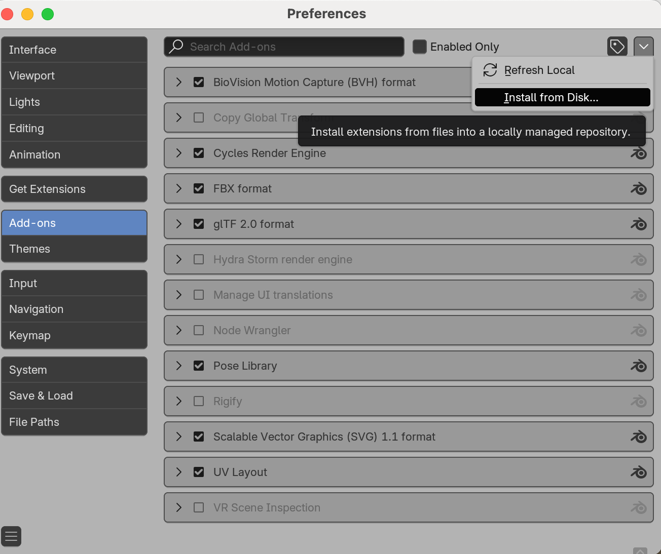
Figure 5:Install the Add-on to Blender.
Now you should see the UI in Figure 4. Fill in the parameters (you can use the given assets from GitHub). Note that you can continue adding more objects to scatter by clicking on “Add Prototype” button. When everything is filled, click “Run USD Scatter” to generate a new USD file with randomized object placement.
Here are some tips for testing: - Start with a low number of instances (like 10–20) to test quickly.
- If nothing appears, double-check file paths, prim paths, and that prototypes are loaded correctly.
If something doesn’t work the first time, don’t worry! Here’s a checklist to help you diagnose common issues when installing or running the USD Object Scatter add-on: 1. Add-on Installation - Did you zip the folder, not just the files inside it? Blender expects a .zip file with a top-level folder (e.g., usd_scatter_addon/). - Is init.py at the top level of the folder? Blender won’t detect your add-on unless this file is directly inside the zipped folder. - Is the add-on showing up in Preferences > Add-ons? If not, check the bl_info block for syntax errors or missing commas.
  2. File and Path Issues
  - Are your file paths correct and accessible? If the USD files or textures are on an external drive or have spaces in names, make sure the full paths are valid.
  - Are your prim paths correct? For example, /World/Rock1 must exactly match the path to the object inside the USD file.
  - Do all prototypes have a valid USD file and prim path set? Forgetting to set one will cause the script to fail silently or crash.

  3. Running the Scatter
  - Are Minimum Distance and Bounds reasonable values? If they’re too large, there may not be space to place anything. Try disabling Minimum Distance by setting it to 0

  4. After Running
- Did the output USDA file get saved? Check the folder you specified in Output USDA Path.You now have a complete pipeline — from custom Python code to a usable tool inside Blender, outputting scenes ready for high-end rendering or simulation in the USD ecosystem. Whether you’re an artist, TD, or engineer, this foundation is one you can build on.
12.5 Closing Thoughts
With this, you’ve reached the end of OpenUSD in One Weekend. Throughout this book, we’ve explored how USD works under the hood — not just as a file format, but as a flexible, programmable scene graph that can support animation, physics, AI-assisted workflows, and scalable content pipelines.
We’ve moved from foundational concepts to practical tools — from defining simple prims to building a Blender add-on that artists can use out of the box. Along the way, you’ve developed a deep working knowledge of the USD Python API, structured reusable code, and hopefully discovered new ways to combine code and creativity.
Whether you’re a developer, TD, pipeline engineer, or artist exploring automation, you now have the tools to continue building with USD — not just using it, but extending it to meet your own needs.