This appendix covers
- Downloading and installing Blender
- Using Blender Python API for basic scene operations
- Rendering in Blender
- Playing with the Physics Simulation in Blender
B.1 Getting Started with Blender
Blender (https://
Developers can script automation and integration through Blender’s Python API (https://
Blender has growing integration with OpenUSD, for describing, composing, and exchanging 3D assets and scenes. OpenUSD’s focus on interoperability aligns perfectly with Blender’s mission to support open standards in the 3D content creation ecosystem.
Getting started with Blender is quick and straightforward:
- Download: Visit the official Blender website and navigate to the Download page (https://
www .blender .org /download/). - Install: choose the version compatible with your operating system (Windows, macOS, or Linux) and get started!
B.2 The Basics of Blender’s Python API
Blender’s Python API is a powerful scripting interface that allows users to automate tasks, customize workflows, and extend Blender’s functionality through Python programming. With access to nearly all of Blender’s features, the API enables programmatic control over modeling, animation, rendering, physics simulations, and more. By using the Python API, you can efficiently handle repetitive tasks, create procedural assets, develop custom tools, and integrate Blender into larger pipelines. This level of flexibility and control makes the Blender Python API an indispensable tool for users looking to enhance productivity, streamline complex workflows, and unlock new creative possibilities.
After installing and opening Blender, Figure 1 shows how to open the console to start coding. At the top of the screen the navigation bar offers a variety of tabs that provide interface layouts that are optimized for specific tasks. Let’s select the ‘Scripting’ tab, which will rearrange the layout of the standard interface, and open two additional windows, the Text Editor, and the Python Console.
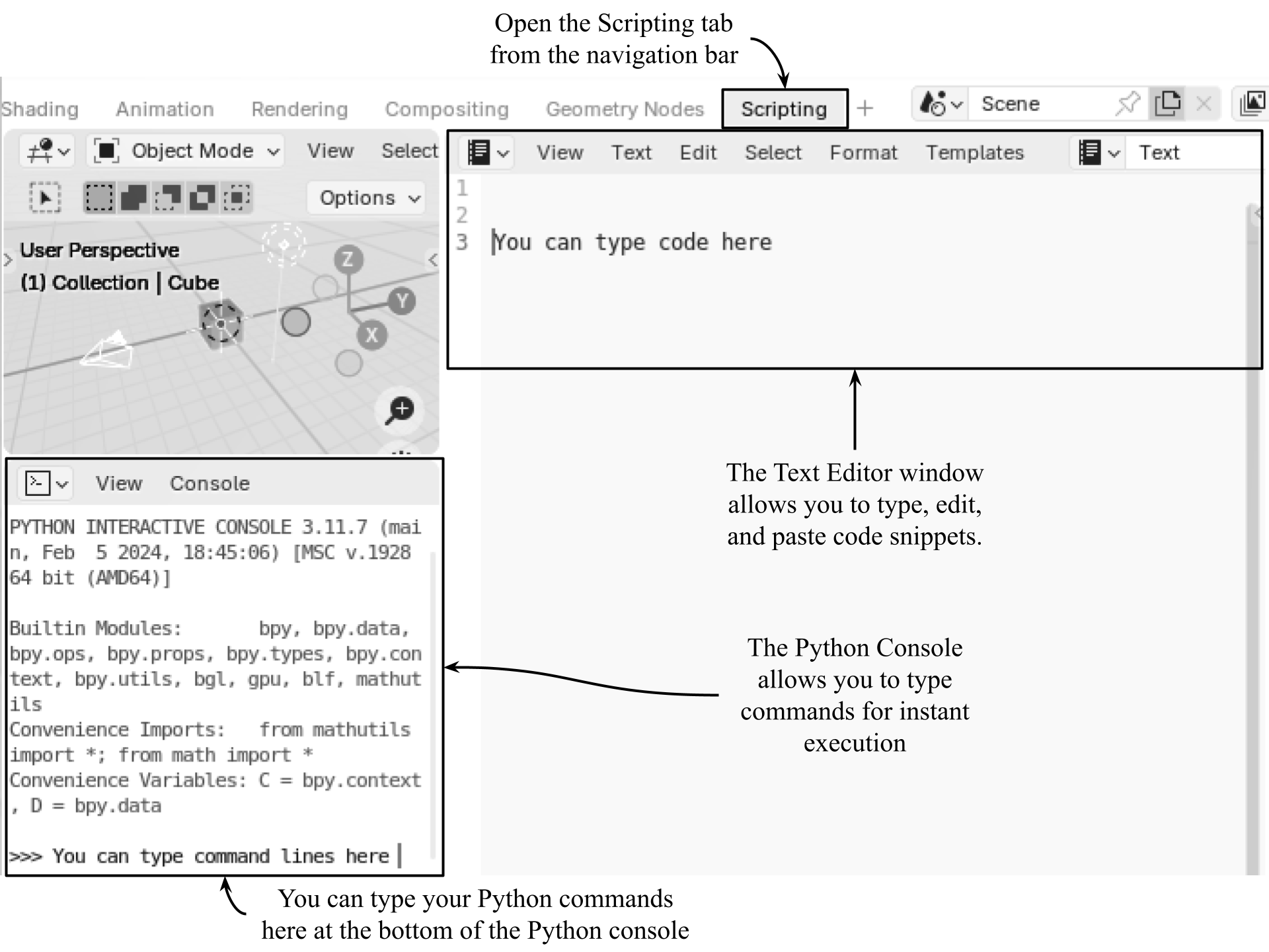
Figure 1:Opening Blender’s Scripting tab on the navigation bar provides an interface optimized for scripting. The Python Console on the bottom left helps to interactively execute your commands one line at a time. The Text Editor on the right is where you can compose and execute a longer code snippet.
Text Editor
This window is where you write and edit your Python scripts. Think of it as a standard text editor, but tailored for Python code within Blender. You can save your scripts as external .py files, load existing scripts, and organize them. It provides syntax highlighting, which helps you identify different parts of your code (keywords, variables, etc.), making it easier to read and debug.
To use the text editor:
- In the Text Editor window, click Text → New to create a new script.
- Type or paste your Python code into the editor.
- Click the Play symbol (▶️) in the top bar of the window, or press Alt + P to execute the script.
- If needed, save your script using Text → Save As...
Python Console
This is an interactive shell where you can type Python commands and see immediate results. Just like the command terminals we’ve been using elsewhere in the book, pressing enter will instantly execute a command. It is useful for testing small snippets of code before adding them to a full script, inspecting the current state of your Blender scene, quickly accessing and modifying Blender data, and seeing the output of print statements from scripts run in the text editor.
To use the python console:
- In the Python Console, type a command and press Enter.
- The output appears immediately in the console.
- Use the up/down arrow keys to navigate through previous commands.
- Use Blender’s Python module (bpy) to interact with Blender’s data and functionality, i.e., bpy.data.objects to list objects in the scene.
Let’s test it out by opening a new stage in Blender. It will open with the default cube, light and camera. In the Python Console, let’s change the working directory in the usual way:
import os
working_directory = '<your_usd_file_path>'
os.chdir(working_directory)

# Import Blender's Python module
import bpy

# List all the objects in the current scene
list(bpy.data.objects)
Now, let’s clear the stage of all existing objects so that we can start building a new scene from scratch. The following snippet will traverse through all objects, then remove them:
# Traverse all the objects
for obj in bpy.data.objects:
    # Remove all the objects
    bpy.data.objects.remove(obj, do_unlink=True)
Note Sometimes the Python Console on Windows (or with certain editors) treats empty lines as block terminators when pasting, causing an “unexpected indent” error. If this happens try pasting the code without blank lines between function lines.
B.2.1 Creating Basic Geometries
To create basic geometries such as cubes, spheres, and cylinders using Blender’s Python API, you can use the bpy.ops.mesh.primitive_* operators. You can specify the location, rotation, and size of it while creating the object. Each type of primitive expects certain parameters to be set, otherwise default values are used.
For example, calling bpy.ops.mesh.primitive_cube_add() without parameters will place a cube at (0,0,0) with a size of 2 Blender units. Here’s a quick examples for adding a cube with specified parameters:
# Create a cube mesh and set its size, location, and rotation
bpy.ops.mesh.primitive_cube_add(size=2, location=(-1.5, 2, 1), rotation=(0, 0, 30))
Similarly, you can also add an ico sphere and a cone. Notice that the sphere expects a radius, and the cone requires two radii, one for the base and one for the tip, and a depth, which determines the height of the tip:
bpy.ops.mesh.primitive_ico_sphere_add(radius=1, location=(-0.3, -1.5, 1), subdivisions=4)

bpy.ops.mesh.primitive_cone_add(vertices=32, radius1=1.0, radius2=0.0, depth=2.0, location=(1.5, 0.5, 1.0), rotation=(0.0, 0.0, 0.0))
For different geometries, you may need to check which parameters are expected. We recommend readers to refer to the Blender Mesh Operation documentation here: https://
The API provides access to nearly all the controls available in the GUI. For example, the ‘Shade Smooth’ option, typically found under the ‘Object’ menu, can also be applied through scripting. Let’s use it to make the Ico Sphere look smoother.
The following snippet ensures that the “Icosphere” object is properly selected and active before applying smooth shading. First, it deselects all objects to prevent unintended modifications. Then, it selects “Icosphere” and sets it as the active object , which is required for many bpy.ops operations. Finally, it applies smooth shading to create a smoother appearance:
# Deselect all objects
bpy.ops.object.select_all(action='DESELECT')

# Select the Ico Sphere
bpy.data.objects["Icosphere"].select_set(True)

# Set the Ico Sphere as the active object
bpy.context.view_layer.objects.active = bpy.data.objects["Icosphere"]

# Apply Shade Smooth to the active object
bpy.ops.object.shade_smooth()
The ico sphere should now appear smooth in the viewport.
B.2.2 Importing Objects
Blender supports importing various file formats, each with its own method. Each format has a specific import operator under bpy.ops.import_scene. For example, we could import an .fbx file using bpy.ops.import_scene.fbx(filepath=“/path/to/your/file.fbx”). This method will work for most file formats by using the relevant operator, ‘import_scene.fbx’ for fbx, ‘import_scene.gltf’ for glb, etc.
However, importing .usd and .obj files is slightly different as it requires us to use the Window Manager Operations (bpy.ops.wm). For example, we could import an .obj file using bpy.ops.wm.obj_import(filepath=“/path/to/your/file.obj”).
Let’s apply this by importing an object into our current scene. We’ll use the ‘backdrop.usd’ that we have provided in the ‘Assets’ folder for this Appendix. If you don’t have it already, you can find it on our GitHub repo here: https://
Run the following line in Blender to import the backdrop.usd:
# Imports the 'backdrop.usd' from the Assets folder
bpy.ops.wm.usd_import(filepath=<your_usd_file_path> ex: './Assets/backdrop.usd'>)
For more information on the window manager module check: https://
By now, you might be starting to recognize this scene as the ‘Hello_World’ scene we used in Appendix A. Let’s continue to build it by adding a camera.
B.2.3 Adding a Camera
To add a camera let’s use the bpy.ops.object.camera_add() method, setting its location and rotation. Blender’s bpy.ops.object.camera_add() expects rotation values in radians, not degrees, so we’ll need to utilize Python’s math module if we want to replicate the 80° rotation of the camera in the original ‘Hello_World’ scene.
Luckily, as we know we want the camera rotated by 80° around the x axis, we can use the math module to convert degrees to radians using math.radians(), as follows:
import math

# Add a camera and set its location and rotation, converting degrees into radians
bpy.ops.object.camera_add(location=(0, -10, 3), rotation=(math.radians(80), 0, 0))

# Set the camera as the active object
camera = bpy.context.active_object
Next, let’s adjust the camera properties using camera.data, which gives access to settings like focal length, depth of field, and aperture. Since we’ll be modifying properties that affect the depth of field (DOF), we’ll also enable the use_dof setting by setting it to ‘True’:
camera.name = "Camera_1"

# Set the focal length
camera.data.lens = 50

# Enable depth of field
camera.data.dof.use_dof = True

# Set the focus distance
camera.data.dof.focus_distance = 10

# Set the F-stop value
camera.data.dof.aperture_fstop = 2.8
Currently, our stage is dark, so let’s add some lights.
B.2.4 Introducing Lighting
Adding lighting in Blender using Python involves creating a light object, specifying its type (i.e., point, sun, spot, or area), location,and rotation. The scale of a light can also be set, but this is not recommended. It is preferable to adjust the size of a light after it has been created by adjusting its ‘size’ property.
Let’s add an Area Light to our stage making sure to name, locate, and rotate it as we add it. Then, we can adjust the Power property of the light’s data block using light.data.energy:
bpy.ops.object.light_add(
    # Set the type to 'AREA'
    type='AREA',

    # Set location
    location=(2, -3, 4),

    # Rotation in radians (each 45° rotation converted)
    rotation=(math.radians(45), 0, math.radians(45))
)

# Reference the newly added object
main_light = bpy.context.object

# Rename it to 'Main_Light'
main_light.name = "Main_Light"

# Set light energy to 150 watts
main_light.data.energy = 150
Let’s add a second light to lighten the shadows being thrown by the Main Light. We’ll call this one ‘Side_Light’:
bpy.ops.object.light_add(
    # Set the type to 'AREA'
    type='AREA',

    # Set location
    location=(-6, 2, 1),

    # Rotation in radians (90° rotation converted)
    rotation=(0, math.radians(-90), 0)
)

# Reference the newly added object
side_light = bpy.context.object

# Rename it to 'Side_Light'
side_light.name = "Side_Light"

# Set light energy to 50 watts
side_light.data.energy = 50
Now, if we change the viewport shading method to ‘Rendered’, we will see the effect of our two new lights. (For instructions on how to do this, refer to Figure 16.
B.2.5 Applying Materials
To complete this scene, let’s learn how to create and apply materials. We can start by creating a green color for the backdrop. The first snippet in this subsection will create a material named “Green”, defining its color using RGBA values. It then enables the use of shader nodes and modifies the Principled BSDF node parameters for Base Color and Roughness. Finally, it finds the Backdrop object and assigns the material:
# Define RGBA color (Alpha = 1)
green = (0.58, 0.8, 0.59, 1)

# Create a new material named "Green"
green_mat = bpy.data.materials.new(name="Green")

# Enable shader nodes
green_mat.use_nodes = True

# Get the Principled BSDF node
bsdf = green_mat.node_tree.nodes.get("Principled BSDF")

# Set base color
bsdf.inputs["Base Color"].default_value = green

# Set roughness
bsdf.inputs["Roughness"].default_value = 0.5

# References the Backdrop object
backdrop = bpy.data.objects["Backdrop"]

# Remove any existing materials from the backdrop
backdrop.data.materials.clear()

# Assign the new material
backdrop.data.materials.append(green_mat)

# References the Ground object
ground = bpy.data.objects["Ground"]

# Remove any existing materials from the ground
ground.data.materials.clear()

# Assign the new material
ground.data.materials.append(green_mat)
Next lets automate the process of creating and assigning materials to objects. First we’ll define a function, create_material(), which generates a new material with a specified name and color, enabling shader nodes and setting the Base Color and Roughness properties. Then we’ll define RGB color values corresponding to blue, yellow, and red. Next, we’ll create three materials—one for each color—and store them in a dictionary mapped to object names. Finally, we’ll iterate through the dictionary, assigning the appropriate material to each object (Cube, Icosphere, and Cone). If an object has no material, the script adds one; otherwise, it replaces the existing material. This approach ensures a structured and reusable way to apply materials without manually modifying each object:
def create_material(name, color):
    """Create a new material with the specified name and RGB color."""

    # Create a new material and assign it a name
    mat = bpy.data.materials.new(name=name)

    # Enable shader nodes for the material
    mat.use_nodes = True

    # Get the Principled BSDF node
    bsdf = mat.node_tree.nodes.get("Principled BSDF")

    # Set Base Color
    bsdf.inputs["Base Color"].default_value = (*color, 1)

    # Set Roughness
    bsdf.inputs["Roughness"].default_value = 0.5

    # Return the created material
    return mat


# Define RGB colors
blue = (0.4, 0.46, 0.91)
yellow = (0.88, 0.91, 0.34)
red = (0.91, 0.39, 0.35)


# Create materials and assign them to corresponding objects
materials = {
    # Create a blue material for the Cube
    "Cube": create_material("Blue_Mat", blue),

    # Create a yellow material for the Icosphere
    "Icosphere": create_material("Yellow_Mat", yellow),

    # Create a red material for the Cone
    "Cone": create_material("Red_Mat", red)
}


# Iterate through the materials dictionary
for obj_name, mat in materials.items():
    # Get the object by name
    obj = bpy.data.objects.get(obj_name)

    if obj:
        if not obj.data.materials:
            # Add material if none exists
            obj.data.materials.append(mat)
        else:
            # Replace existing material
            obj.data.materials[0] = mat
The stage should now look just like the ‘Hello_World’ usd file we used in Appendix A. Next let’s consider how we would render an image from this scene.
B.3 Rendering with Blender’s Python API
The rendering process transforms 3D models, lights, and materials into 2D images. This involves complex calculations simulating how light interacts with objects in the scene, considering factors like shadows, reflections, and refractions. Blender offers two primary rendering engines:
- Eevee: A real-time renderer providing fast feedback during modeling and animation.
- Cycles: A physically-based path tracer known for its photorealistic results, but requiring more computational power.
By adjusting render settings like resolution, sampling, and denoising, users can fine-tune both the quality and appearance of their final output, as well as improve the efficiency of the rendering process. To make the most of the Cycles renderer, we’ll focus on adjusting the following settings for optimal performance:
- Sampling: Determines the number of rays traced per pixel. Higher values produce cleaner images but increase render time. We’ll balance quality and performance by setting a reasonable sample count (e.g., 128-256 for final renders, lower for previews).
- Adaptive Sampling: Adjusts the sample count per pixel dynamically, reducing noise where fewer samples are needed. Enables faster rendering by focusing computation on noisy areas while skipping unnecessary samples. We’ll enable it to optimize performance without sacrificing quality.
- GPU Compute: Uses the GPU instead of the CPU for rendering, significantly improving speed on supported hardware. (Must be enabled in Preferences → System → Cycles Render Devices before setting it in the script. We can use “CUDA”, “OPTIX”, or “HIP” depending on our GPU type.)
- Denoising: Reduces noise in the final image without needing excessive samples, improving render speed.
Each of these settings works together to balance speed and quality, making Cycles rendering more efficient.
Let’s render an image from our new ‘Hello_World’ scene. First, we will set the camera to active and specify the file path where the rendered image will be saved. Note that the file extension will determine the output format of the image (i.e., .png, .jpeg), and that copy/pasted file paths may need the ‘r’ prefix to prevent Python using the backslashes as escape characters.
With the camera and file path set, next let’s define the resolution of the output image and set the render engine to Cycles using bpy.context.scene.render.engine = ‘CYCLES’. (For Eevee, we would use ‘BLENDER_EEVEE’).
To optimize both the rendering speed and the final output, we can adjust the sampling settings, enable adaptive sampling, and switch to GPU rendering for faster performance. Next, we can enable denoising to reduce noise and improve the visual quality of the render. Finally, we can trigger the rendering process and save the result using bpy.ops.render.render(write_still=True). There will be a pause after running this final line, as the computation of the renderer will have begun:
# Get Camera_1
camera = bpy.context.scene.objects.get("Camera_1")

# Set the camera to active
bpy.context.scene.camera = camera

# Set your image path (note the use of the r prefix to denote raw strings)
bpy.context.scene.render.filepath = r"<your/path/to/save/image ex: C:\\Appendix_B\Hello_World_Render.png"

# Set the output resolution
bpy.context.scene.render.resolution_x = 1920
bpy.context.scene.render.resolution_y = 1080

# Set the render engine to Cycles
bpy.context.scene.render.engine = 'CYCLES'

# Set the sample rate to 128
bpy.context.scene.cycles.samples = 128

# Enable adaptive sampling for extra efficiency
bpy.context.scene.cycles.use_adaptive_sampling = True

# Enable GPU for faster rendering
bpy.context.scene.cycles.device = 'GPU'

# Enable denoising in Cycles
bpy.context.scene.cycles.use_denoising = True

# Render and save the image (expect a pause before output)
bpy.ops.render.render(write_still=True)
Once the render has finished computing the final output, you should see a {‘FINISHED’} message in your console. Now you can go to your output folder to view the rendered image. It should look like Figure 2.
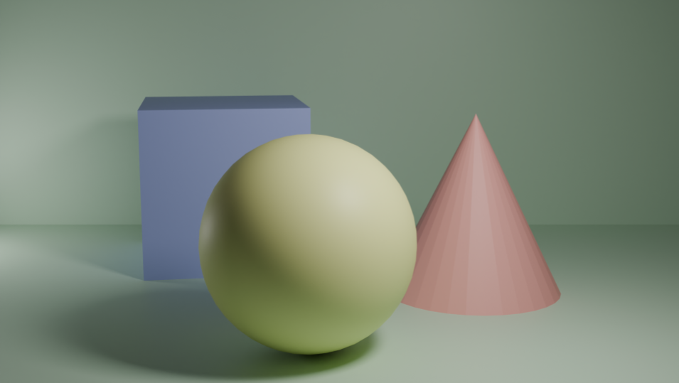
Figure 2:The expected output from the render of our ‘Hello_World’ scene.
Scripting the rendering process in Blender streamlines repetitive tasks and enhances efficiency by automating settings such as resolution, output paths, and render engine configurations. This approach can save time and ensure consistency, making it especially valuable in professional environments like animation studios or product visualization, where multiple, large-scale renders are often needed. Automation enables batch processing and precise control, ultimately speeding up workflows and improving productivity.
B.4 Simulating Physics in Blender
If you are using Blender to explore OpenUSD you have probably arrived here from Chapter 8, where we discuss physics simulations. As OpenUSD uses the PhysX engine and Blender uses a mix of physics engines, the code we presented there is not applicable for Blender users. However, we can still utilize Blender’s physics capabilities with imported .usd files, so we have added this section specifically for that purpose. Even if you can’t run the code in Chapter 8, reading it is still valuable. The core concepts and terminology related to physics engines are broadly applicable, and will help you understand the principles applied here.
Blender uses the open-source Bullet Physics Library for rigid body simulations and Mantaflow for fluid dynamics. Just as Python scripts control OpenUSD/PhysX through its pxr API, they can also manage Blender’s physics via the bpy API. In both cases, Python acts as an intermediary, adjusting the API to direct the physics engine.
Figure 3 shows the stage we’ve provided containing a cube, a sphere, and a ground plane so that we can start creating a physics simulation.
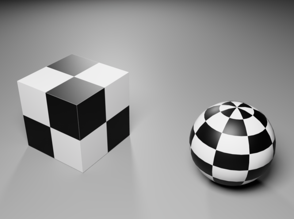
Figure 3:The ‘physics.usda’ stage showing the cube and sphere that we will use to demonstrate basic physics.
Let’s begin by opening a new stage in Blender, switching to the Scripting tab, and removing the default objects:
import bpy

# Traverse all the objects
for obj in bpy.data.objects:
    # Remove all the objects
    bpy.data.objects.remove(obj, do_unlink=True)
Now let’s import the ‘physics.usda’ file, and list all of the objects on the stage so that we know what names we are going to work with later. We don’t need to list all the lights and materials, so let’s set up a filter to list only meshes by using if obj.type == ‘MESH’:
# Imports the 'physics.usda' from the Assets folder
bpy.ops.wm.usd_import(filepath="<your_path_to_physics.usda>" )  # Example: './physics.usda'

# Filter only mesh objects
mesh_objects = [obj for obj in bpy.data.objects if obj.type == 'MESH']

# Print the names of the filtered mesh objects
print([obj.name for obj in mesh_objects])
This list should return this list: “[‘CollisionMesh’, ‘Cube_mesh’, ‘Sphere_mesh’]”. Note that the object named ‘CollisionMesh’ is the ground plane.
Next, let’s add a Rigid Body to the Cube_mesh, which will allow us to set some of its physics properties such as Mass, Friction, and Restitution. For a detailed discussion on how these properties affect an object, please refer to the relevant sections of Chapter 7. We will also need to consider whether we want the rigid body to simulate an active object (one that moves and is affected by forces like gravity or collisions), or a passive object (one that remains stationary, like a floor or wall, but still creates collisions). For this we have the option of using a string literal to set the rigid body type as either ‘ACTIVE’, or ‘PASSIVE’.
Let’s get the Cube-mesh, and apply those properties as follows:
# Get the cube
cube = bpy.context.scene.objects.get("Cube_mesh")

# Set the cube as the active object
bpy.context.view_layer.objects.active = cube

# Select the cube
cube.select_set(True)

# Add the rigid body to the Cube_mesh
bpy.ops.rigidbody.object_add()

# Set the rigid body type to 'ACTIVE'
cube.rigid_body.type = 'ACTIVE'

# Set the rigid body's Mass, Friction, and Restitution values
cube.rigid_body.mass = 1
cube.rigid_body.friction = 0.5
cube.rigid_body.restitution = 1.0
Note Blender will apply bpy.ops.rigidbody.object_add() to the active object, even if it is not selected using the line cube.select_set(True). However, we include this here as in some cases, certain operators require selection, so it’s a good habit to ensure both selection and active status when using bpy.ops.
Now is a good time to test the simulation by running it. In Blender, a physics simulation is started and stopped in the same way as an animation using:
# Starts an animation or physics simulation
bpy.ops.screen.animation_play()
When building a simulation scene it is often preferable to open a Timeline window from the drop down Editor Type menu found at the top left of any window in Blender, as this gives easy access to Play/Pause/Return to Start type controls. If you are unsure of how to do this, please refer to Figure 6.2 in Chapter 6. Alternatively, you can use hotkeys: the Space bar to start or stop the simulation, and Shift + Left Arrow to reset it to the starting point.
If you have run the simulation, you will have observed the cube falling through the ground. If you let the simulation run for long enough, it will loop through the number of frames set on the timeline (default is 100), then the simulation returns to its starting state and runs again. If we need the simulation to run for longer, we can increase the number of frames in the simulation by adjusting the end frame:
# Set the end frame to 250
bpy.context.scene.frame_end = 250
We have demonstrated how to add a rigid body to a single object, but sometimes we might want to add rigid bodies to multiple objects at once, and set their properties at the same time. Let’s explore how to do that by working with the other two meshes on our stage.
The following snippet will create a list of the objects we want to apply rigid bodies to, then use bpy.ops.rigidbody.object_add() and obj.rigid_body.* in a loop:
# List of meshes to add rigid bodies to
mesh_names = ["CollisionMesh", "Sphere_mesh"]

for name in mesh_names:
    # Get the object by name
    obj = bpy.context.scene.objects[name]

    # Set as the active object
    bpy.context.view_layer.objects.active = obj

    # Add the rigid body
    bpy.ops.rigidbody.object_add()

    # Set the same Mass, Friction, and Restitution on all objects in the loop
    obj.rigid_body.mass = 1
    obj.rigid_body.friction = 0.5
    obj.rigid_body.restitution = 1
Playing the simulation now will reveal a problem: The ground plane (‘Collision_mesh’) is being affected by gravity and falls away with the cube and sphere. To fix this, we need to change the Collision_mesh’s rigid body type to Passive. This will keep it unaffected by forces while still allowing it to interact with collisions:
# Set the Collision_mesh object
collision_mesh = bpy.context.scene.objects["CollisionMesh"]

# Set the rigid body type to Passive
collision_mesh.rigid_body.type = 'PASSIVE'
Running the simulation now will show that the ground behaves as expected and stays in place. However, the cube and sphere remain stationary because no force is acting on them. In USD Composer, we can grab and move objects during the simulation, but this functionality isn’t currently available in Blender. Therefore, to demonstrate how these objects will behave when they collide, let’s adjust their starting positions so they are in the air and will fall when the simulation is run:
# Set Cube_mesh position
bpy.context.scene.objects["Cube_mesh"].location = (-300, 0, 600)

# Set Sphere_mesh position
bpy.context.scene.objects["Sphere_mesh"].location = (100, 100, 900)
Now when the simulation runs, you will see the objects fall, collide with the ground, and bounce due to the high restitution value we have given them. We encourage you to have fun and experiment by trying out different property settings, such as higher mass, or less restitution.
It is also possible to set the gravity and rigid body world as active or inactive using the following methods. Setting the rigid body world to inactive will disable any rigid body dynamics if necessary:
# Set gravity to standard on Earth
bpy.context.scene.gravity = (0, 0, -9.81)

# Enable the rigid body world (set to False to deactivate rigid body dynamics)
bpy.context.scene.rigidbody_world.enabled = True
By default, Blender already has gravity set to (0, 0, -9.81), which is the standard gravity on Earth, and the rigid body world is enabled. You would only need to explicitly set these properties if you want to modify gravity or ensure the rigid body world is enabled after being disabled for some reason. If everything is functioning as expected, these lines aren’t necessary.
We have demonstrated the fundamentals of using Blender’s Python API to control physics simulations, demonstrating how to import .usd files, apply rigid bodies to them, and adjust their physics properties. While this chapter focused on the essentials, Blender offers a wide range of advanced simulation tools beyond rigid body dynamics. In the final section, we will touch on some of these additional simulation types, though an in-depth exploration is beyond the scope of this Appendix. We encourage you to experiment further and take full advantage of Blender’s powerful physics engine.
B.5 Introducing Other Simulations
Blender offers a variety of physics simulations beyond rigid bodies to create more complex and realistic animations.
- Cloth simulation allows for the realistic behavior of fabrics, where objects such as clothes or flags can respond to forces like wind, gravity, and collision with other objects. The simulation accounts for stretching, bending, and friction between the cloth and other surfaces, making it ideal for creating dynamic and flowing fabrics.
- Soft Body physics simulates objects that deform and bend under forces, such as jelly or rubber materials. It allows objects to maintain their shape while reacting to external forces, providing a more flexible and organic response compared to rigid body simulations.
- Particle systems in Blender enable the simulation of small particles, such as dust, smoke, fire, and rain. These particles can be controlled through various forces, like wind, gravity, and turbulence, creating dynamic effects that interact with the environment.
- Fluid simulation provides a way to simulate the behavior of liquids, allowing for the creation of realistic water flow, splashes, and interactions with solid objects. Fluid simulations can be set up for both liquid-to-liquid and liquid-to-gas interactions, giving animators the tools to simulate everything from water pouring into a container to large-scale ocean simulations. These simulations add a layer of realism and interactivity, essential for creating visually convincing animations and special effects.
For more details, readers can refer to the official documentation (https://